Download
1 / 32
330 likes | 451 Views
Scientific Visualization An Introduction. Michel O. R. Eboueya Computer Sciences Department Pôle Sciences et Technologies Université de La Rochelle. Outline. Introduction: Definitions, Goals and History of Visualization Part 1 Visualization Concepts

E N D
Scientific Visualization An Introduction Michel O. R. Eboueya Computer Sciences Department Pôle Sciences et Technologies Université de La Rochelle
Outline • Introduction: Definitions, Goals and History of Visualization • Part 1 • Visualization Concepts • Characterization of data and Short Vocabulary • Algorithms (Scalars, Vectors, Direct volume rendering ) • Part 2 • Visualization Techniques • Advanced topics (Virtual reality,Texture ) • Scientific Visualization Tools (Some commonly used programs ) • Conclusion
Algorithms Scalar Algorithms Color Mapping Contouring (contour tracking, Marching squares, cubes…) scalar generation Vector Algorithm Hedgehog and Oriented Glyphs Warping Displacement Plots Time Animations Streamlines Modeling Algorithms Implicit Functions Glyphs Cuttings
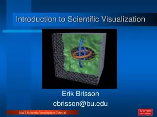
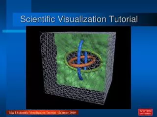
Volume de visualisation Volume Visualization(3d domain): Displays volumetric (3D-mesh) data by showing a color, greyscale or object at every grid point. Usually uses transparency to show as much data as possible.
DVR Algorithms • Data Classification for Volume Visualization • Surface-fitting: • User Picks Threshold Value • Direct Volume Rendering: • User Specifies Color Table Map Data Values to Meaningful Colors • User Specifies Opacity Table Map Interesting Data to Opaque • Map Other Data to Transparent • Setting up the Tables
DVR Algorithms Data Classification for Volume Visualization
Direct ScVs Al. • ray-castingA volume viewing algorithm in which sight rays are cast from the viewing plane through the volume. The tracing of the ray stops when the visible voxels are determined by accumulating or encountering an opaque value. [KAU91] • ray-tracing The general technique of computing an image by projecting rays into a scene and using their interactions with the contents of that scene to determine pixel colors. In surface- rendering methods, rays are intersected and possibly reflected or refracted by objects in the scene to determine visible colors. Ray-tracing is also used in volume visualization and is a type of DVR. [WOL93]
Object Based Rendering: Ray Tracing http://gandalf.iuk.tu-harburg.de/hypgraph/raytrace/rtrace1.htm
DVR Algorithms Ray Casting (Image-order methods) Ray-casting Methods Basic Idea • Cast Rays from Image Plane through Volume to Find Pixel Color • No Intermediate Surfaces • Renders Volume Directly Ray-casting Fundamentals: Brute Force Algorithm • For each Pixel • For each f(i,j,k) Along a Ray from Pixel • Check f(i,j,k) in Classification Tables • If New Substance • Find Surf Normal/Compute Color • Weight Color by Opacity • Accumulate Color Contribution and Opacity • Pixel Gets Accumulated Color
DVR Algorithms Ray-casting Advantages • No Binary Classification, e.g., inside or outside as in surface fitting methods • Shows Structure Between Surfaces • Displays Small and Poorly Defined Features • Readily Parallelizes Ray-casting Disadvantages • Expensive - Cost Proportional to Volume Size (N^3) • Combining Geometry and Volume Data is Difficult Rendering Methods and Hardware are Unknown
Volume Rendering • Displays all of the 3-D data at once, like an X-ray: Denser parts are more opaque. • User controls the density of various data values.
DVR Algorithms Ray-casting Example Dolphin head (Cranford, Elvins, Mercurio)
Projection methods in DVR Ray Casting • Ray-casting is the most used algorithm for the generation of high quality images. It performs an image-order traversal of the image plane pixels, determining a color and opacity for each pixel. A ray is fired from the center of each pixel through the volume. The colors and opacities are summed along each ray and the result is used to shade the pixel. The ray continues until it exits the volume or until the sums become greater than one. • The first step is for the user to set up color and opacity tables as discussed in the data classification section. The user then sets the viewing and lighting (if any) information. The ray-caster starts firing rays through the pixels. When a cell is intersected between gridpoints, an interpolation scheme can be used to determine the data value, or for voxel-based rendering the value at the central grid point can be used. Based on this value a color and opacity is assigned from the look up tables. The color and opacity values are modified by the surface gradients, weighted, and then added to the previous values for the ray. Usually values closer to the front are given a higher weighting. The ray then continues through the volume. • Ray-casting is very cpu-intensive but the images can show the entire data set and not just a particular surface. Also, this algorithm can be easily parallelized.
Projection methods in DVR Splatting • Splatting • Splatting performs a front-to-back object-ordered traversal of the voxels in the dataset. Each voxel's contribution to the image is computed and added to the other contributions. • The first step is to determine in what order to traverse the volume. The closest face (and corner) to the image plane is determined. Then the closest voxels are splatted first. Each voxel is given a color and opacity according to the look up tables set by the user. These values are modified according to the gradient. • Next the voxel is projected into image space. To compute the contribution for a particular voxel, a reconstruction kernel is used. For an orthographic projection a common kernel is a round Gaussian. The projection of this kernel into image space (called its footprint) is computed. This size is adjusted according to the relative sizes of the volume and the image plane so that the volume can fill the image. Then the center of the kernel is placed at the center of the voxel's projection in the image plane (note that this does not necessarily correspond to a pixel center). Then the resultant shade and opacity of a pixel is determined by the sum of all the voxel contributions for that pixel, weighted by the kernel. • A voxel's contribution is high near the center of its projection and lower when far from the center. This is sort of like the splat a snowball makes when thrown against a wall. Depending upon the relative sizes of the volume and image plane, several voxels may contribute to a single pixel or a single voxel may contribute to several pixels.
Splatting • The term splatting derives from the analogy with throwing snowballs at a glass plate. The contribution of an individual snowball is higher nearer its center and gradually tails of towards the edges. This is reflected in splatting in the filter used to calculate the contributions of the voxels to the final images. • Splatting has similar advantages and disadvantages to the standard volume rendering techniques. • However it does have an additional advantage that it is possible for the user to see the image growing one slice at a time, rather than one pixel at a time as with the ray casting technique.
Splatting Splatting Example Dolphin Head (Cranford, Elvins, Mercurio)
Algorithms Scalar Algorithms Color Mapping Contouring (contour tracking, Marching squares, cubes…) scalar generation Vector Algorithm Hedgehog and Oriented Glyphs Warping Displacement Plots Time Animations Streamlines Modeling Algorithms Implicit Functions Glyphs Cuttings
Implicit Functions • Modéliser les structures moléculaires avec leur champs d'électrons[. • La mécanique quantique représente la répartition des électrons au sein d'un atome en tant que fonction de densité dans l'espace tridimensionnel. Cette fonction donne la densité en un point donné : • D(x, y, z) = exp(- a.r) avec r = rayon de l'atome. • A partir de là, on peut exprimer la surface comme étant les points qui satisfont l'équation • D(x, y, z) = T ( 1 ) avec T = seuil. -------------------------------------------------------------------------------M. Eboueya. Algos de la ViSC. Mike@univ-lr.fr
Implicit Functions • En fait, on peut dire que c'est la distance d'un point de la surface à un point du squelette qui détermine. • D(x, y, z) = _( bi exp( -ai.ri )) avec ri = distance de (x, y, z) au centre du i eme atome. • Par définition, on appelle fonction implicite une fonction de la forme f(x ,y, z) = k, où k est une constante arbitraire. on appelle surface implicite une surface dont l'ensemble des points vérifie l'équation S = {P e R3 / f(P)= k}où k est appelé l'isovaleur. -------------------------------------------------------------------------------M. Eboueya. Algos de la ViSC. Mike@univ-lr.fr
Implicit Functions -------------------------------------------------------------------------------M. Eboueya. Algos de la ViSC. Mike@univ-lr.fr
Implicit Functions -------------------------------------------------------------------------------M. Eboueya. Algos de la ViSC. Mike@univ-lr.fr
Implicit Functions -------------------------------------------------------------------------------M. Eboueya. Algos de la ViSC. Mike@univ-lr.fr
Implicit Modeling -------------------------------------------------------------------------------M. Eboueya. Algos de la ViSC. Mike@univ-lr.fr
Glyphs • Glyphs used to indicate normals. • Glyphing is one of the most versatile visualization technique. They are often designed to show many variables simultaneously. The secret of glyph design is simple, an intuitive, relation type between data variable(s) and glyph features.
Cutting • Gas density as fluid flows through a combustion chamber. • The Color correspond to the flow density
Conclusion on Volume Visualization Methods • The fundamental algorithms are of two types: direct volume rendering (DVR) algorithms and surface-fitting (SF) algorithms. • DVR methods map elements directly into screen space without using geometric primitives as an intermediate representation. DVR methods are especially good for datasets with amorphous features such as clouds, fluids, and gases. A disadvantage is that the entire dataset must be traversed for each rendered image. Sometimes a low resolution image is quickly created to check it and then refined. The process of increasing image resolution and quality is called "progressive refinement". • SF methods are also called feature-extraction or iso-surfacing and fit planar polygons or surface patches to constant-value contour surfaces. SF methods are usually faster than DVR methods since they traverse the dataset once, for a given threshold value, to obtain the surface and then conventional rendering methods (which may be in hardware) are used to produce the images. New views of the surface can be quickly generated. Using a new threshold is time consuming since the original dataset must be traversed again.
Vocabulary Cont. • surface modelingTechniques and tools for building up computer representations of objects by modeling their surfaces, usually as a collection of polygonal facets. [WOL93] • surface renderingan indirect technique used for visualizing volume primitives by first converting them into an intermediate surface representation (see surface reconstruction) and then using conventional computer graphics techniques to render them. [KAU91] • surface reconstructionA procedure that converts a set of data points or cross sections into a surface representation by identifying the surface and representing it with geometric surface primitives. The reconstruction procedure may use one of several techniques, such as contouring, tiling, marching cubes, surface detection, and surface tracking. [KAU91]
Vocabulary Cont. • volume renderingVolume rendering is a direct technique for visualizing volume primitives without any intermediate conversion of the volumetric dataset to surface representation. [KAU91] • isosurfaceSurfaces within a volume that have the same parameter value. [WOL93] • Marching CubesA method of visualizing 3-D data structures by looking for level surfaces in a 3-space comprised of a lattice of points. In contrast to volume rendering, where one can see the entire structure, marching cubes only allows a single surface to be rendered. [WOL93]