Download
1 / 48
480 likes | 610 Views
Overview and Introduction to Scientific Visualization. Paul Navratil Texas Advanced Computing Center The University of Texas at Austin Scaling To Petascale Summer School July 9, 2010. Scientific Visualization. “The purpose of computing is insight not numbers.” -- R. W. Hamming (1961).

E N D
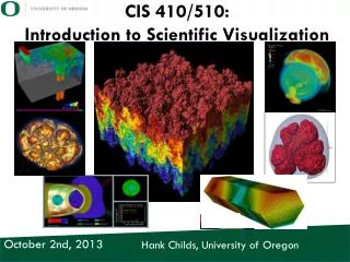
Overview and Introduction toScientific Visualization Paul Navratil Texas Advanced Computing Center The University of Texas at Austin Scaling To Petascale Summer School July 9, 2010
Scientific Visualization “The purpose of computing is insight not numbers.” -- R. W. Hamming (1961)
Visualization Allows Us to “See” the Science Raw Data Geometric Primitives Pixels 01001101011001 11001010010101 00101010100110 11101101011011 00110010111010 Application Render
Getting from Data to Insight Data Representation Visualization Primitives Graphics Primitives Display Iterationand Refinement
“I, We, They” Development Path Simulation Data “I” Data Exploration “We” Collaboration “They” Communication Iterationand Refinement
Visualization Process Summary • The primary goal of visualization is insight • A picture is worth not just 1000 words,but potentially tera- or peta-bytes of data • Larger datasets demand not just visualization, but advanced visualization resources and techniques • Visualization system technology improves with advances in GPUs and LCD technology • Visualization software slower to adapt
Types of Input Data • Point / Particle • N-body simulation • Regular grid • Medical scan • Curvilinear grid • Engineering model • Unstructured grid • Extracted surface
Types of Input Data Point – scattered values with no defined structure
Types of Input Data Grid – regular structure, all voxels (cells) are the same size and shape
Types of Input Data Curvilinear – regularly grided mesh shaping function applied
Types of Input Data Unstructured grid – irregular mesh typically composed of tetrahedra, prisms, pyramids, or hexahedra.
Visualization Techniques • Surface Rendering, is an indirect geometry based technique • Direct Volume Rendering, is a technique for the visualization of 3D scalar data sets without a conversion to surface representations
Visualization Operations • Surface Shading (Pseudocolor) • Isosufacing (Contours) • Volume Rendering • Clipping Planes • Streamlines
Surface Shading (Pseudocolor) Given a scalar value at a point on the surface and a color map, find the corresponding color (and opacity) and apply it to the surface point. Most common operation, often combined with other ops
Isosurfaces (Contours) • Surface that represents points of constant value with a volume • Plot the surface for a given scalar value. • Good for showing known values of interest • Good for sampling through a data range
Volume Rendering Expresses how light travels through a volume Color and opacity controlled by transfer function Smoother transitions than isosurfaces
Clipping / Slicing Planes Extract a plane from the data to show features Hide part of dataset to expose features
Particle Traces (Streamlines) Given a vector field, extract a trace that follows that trajectory defined by the vector. Pnew = Pcurrent + VPDt Streamlines – trace in space Pathlines – trace in time
Visualization Resources • Personal machines • Most accessible, least powerful • Projection systems • Seamless image, high purchase and maintenance costs • Tiled-LCD displays • Lowest per-pixel costs, bezels divide image • Remote visualization • Access to high-performance system, latency can affect user experience
TeraGrid Visualization Resources • Longhorn (TACC) • 256 Nodes, 2048 Total Cores, 512 Total GPUs13.5 TB Aggregate Memory, QDR InfiniBand interconnect • Longhorn Visualization Portal • https://portal.longhorn.tacc.utexas.edu/ • Visualization job submission and monitoring • Remote, interactive, web-based visualization • Guided visualization using EnVision • Spur (TACC) • 8 Nodes, 128 Total Cores, 32 Total GPUs1 TB Aggregate Memory, SDR InfiniBand interconnect • Shares interconnect with Ranger
TeraGrid Visualization Resources • Nautilus (NICS) • SMP, 1024 Total Cores, 16 GPUs4 TB Global Shared Memory, SGI NUMAlink 5 interconnect • Production date: August 1, 2010 • TeraDRE Condor Pool (Purdue) • 1750 Nodes, 14000 Total Cores, 48 Nodes with GPUs28 TB Aggregate Memory, no interconnect
Visualization Allows Us to “See” the Science Raw Data Geometric Primitives Pixels 01001101011001 11001010010101 00101010100110 11101101011011 00110010111010 Application Render
But what about large, distributed data? 01001101011001 11001010010101 00101010100110 11101101011011 00110010111010 01001101011001 11001010010101 00101010100110 11101101011011 00110010111010 01001101011001 11001010010101 00101010100110 11101101011011 00110010111010 01001101011001 11001010010101 00101010100110 11101101011011 00110010111010 01001101011001 11001010010101 00101010100110 11101101011011 00110010111010 01001101011001 11001010010101 00101010100110 11101101011011 00110010111010 01001101011001 11001010010101 00101010100110 11101101011011 00110010111010 01001101011001 11001010010101 00101010100110 11101101011011 00110010111010 01001101011001 11001010010101 00101010100110 11101101011011 00110010111010 01001101011001 11001010010101 00101010100110 11101101011011 00110010111010 01001101011001 11001010010101 00101010100110 11101101011011 00110010111010 01001101011001 11001010010101 00101010100110 11101101011011 00110010111010
Or distributed rendering? 01001101011001 11001010010101 00101010100110 11101101011011 00110010111010
Or distributed displays? 01001101011001 11001010010101 00101010100110 11101101011011 00110010111010
Or all three? 01001101011001 11001010010101 00101010100110 11101101011011 00110010111010 01001101011001 11001010010101 00101010100110 11101101011011 00110010111010 01001101011001 11001010010101 00101010100110 11101101011011 00110010111010 01001101011001 11001010010101 00101010100110 11101101011011 00110010111010 01001101011001 11001010010101 00101010100110 11101101011011 00110010111010 01001101011001 11001010010101 00101010100110 11101101011011 00110010111010 01001101011001 11001010010101 00101010100110 11101101011011 00110010111010 01001101011001 11001010010101 00101010100110 11101101011011 00110010111010 01001101011001 11001010010101 00101010100110 11101101011011 00110010111010 01001101011001 11001010010101 00101010100110 11101101011011 00110010111010 01001101011001 11001010010101 00101010100110 11101101011011 00110010111010 01001101011001 11001010010101 00101010100110 11101101011011 00110010111010
Visualization Scaling Challenges • Moving data to the visualization machine • Most applications built for shared memory machines, not distributed clusters • Image resolution limits in some software cannot capture feature details • Displays cannot show entire high-resolution images at their native resolution
Visualization scales with HPC Large data produced by large simulations require large visualization machines and produce large visualization results Terabytes of Data AT LEASTTerabytes ofVis GigapixelImages Resampling,Application,… Resolution to CaptureFeature Detail
Moving Data • How long can you wait?
Analyzing Data • Visualization programs only beginning to efficiently handle ultrascale data • 650 GB dataset -> 3 TB memory footprint • Allocate HPC nodes for RAM not cores • N-1 idle processors per node! • Stability across many distributed nodes • Rendering clusters typically number N <= 64 • Data must be dividable onto N cores Remember this when resampling!
Imaging Data Hypothetical fly-around movie 4096 x 2160 PNG ~ 10 MB x 360 degrees ~ 3.6 GB x 30 days ~ 108 GB x 12 months ~ 1.3 TB @ 10 fps 3.6 hours @ 60 fps 36 min Image: NASA Blue Marble Project
Displaying Data Dell 30” flat-panel LCD 4 Megapixel display 2560 x 1600 resolution
Displaying Data Stallion – currently world’s highest-resolution tiled display 307 Megapixels 38400 x 8000 pixel resolution Dell 30” LCD
Displaying Data NASA Blue Marble 0.5 km2 per pixel 3732 Mpixel(86400 x 43200) Stallion – 307 Mpixel (38400 x 8000) Dell 30” LCD – 4 Mpixel (2560 x 1600)
Solution by Partial Sums • Moving data – integrate vis machine into simulation machine. Move the machine to data! • Ranger + Spur: shared file system and interconnect • Analyzing data – create larger vis machines and develop more efficient vis apps • Smaller memory footprint • More stable across many distributed nodes Until then, the simulation machine is the vis machine!
Solution by Partial Sums • Imaging data – focus vis effort on interesting features parallelize image creation • Feature detection to determine visualization targetsbut can miss “unknown unknowns” • Distribute image rendering across cluster • Displaying data – high resolution displays multi-resolution image navigation • Large displays need large spaces • Physical navigation of display provides better insights
Old Model (No Remote Capability) Local Visualization Resource HPC System Pixels Mouse Data Archive Display Wide-Area Network Remote Site Local Site
New ModelRemote Capability Pixels Large-Scale Visualization Resource HPC System Display Mouse Data Archive Wide-Area Network Remote Site Local Site
CUDA – coding for GPUs • C / C++ interface plus GPU-based extensions • Can use both for accelerating visualization operations and for general-purpose computing (GPGPU) • Special GPU libraries for math, FFT, BLAS Image: Tom Halfhill, Microprocessor Report
GPU layout Image: Tom Halfhill, Microprocessor Report
GPU Considerations • Parallelism – kernel should be highly SIMD/SIMT • Switching kernels is expensive! • Fermi hardware supports multiple kernel execution • Control Flow – avoid conditionals in kernels • Implemented with predication, harms utilization • Job size – high workload per thread + many threads • amortize thread initialization and memory transfer costs • GPU is a throughput machine, must keep it busy! • Memory footprint – task must decompose well • local store per GPU core is low (16 KB on Tesla) • card-local RAM is limited (1 – 4GB on Tesla) • access to system RAM is slow (treat like disk access)
Summary • Challenges at every stage of visualization when operating on large data • Partial solutions exist, though not integrated • Problem sizes continue to grow at every stage • Vis software community must keep pace with hardware innovations
To learn more about TACC please visit us at:http://www.tacc.utexas.eduThank you!pnav@tacc.utexas.edu