Download
1 / 61
620 likes | 828 Views
Overview and Introduction to Scientific Visualization. Texas Advanced Computing Center The University of Texas at Austin. http://portal.longhorn.tacc.utexas.edu/training. Scientific Visualization. “ The purpose of computing is insight not numbers. ” -- R. W. Hamming (1961).

E N D
Overview and Introduction toScientific Visualization Texas Advanced Computing Center The University of Texas at Austin http://portal.longhorn.tacc.utexas.edu/training
Scientific Visualization “The purpose of computing is insight not numbers.” -- R. W. Hamming (1961)
Visualization Process Summary • The primary goal of visualization is insight • A picture is worth not just 1000 words,but potentially tera- or peta-bytes of data • Larger datasets demand not just visualization, but advanced visualization resources and techniques • Visualization system technology leverages lots of advancing technologies: GPUs, high-speed networks, web technology…. • Visualization software takes time to adapt
Today • Introduction to Visualization • What is scientific data? • Scientific Data Visualization With Paraview • Information Visualization • Remote and Collaborative Visualization • Parallel Visualization For Very Large Data
Visualization Allows Us to “See” the Science Raw Data 01001101011001 11001010010101 00101010100110 11101101011011 00110010111010 Visualization Application
Getting from Data to Insight Data Source Data Representation Visualization Algorithms Rendering Display Computational Steering Refinement Changing Techniques Changing View … And using insight to get more insight
I Think Of Two Kinds Of Data For Visualization… • Data for ‘Scientific Visualization’ • F(spatial dimensions[, time]) -> attributes • E.g. Weather data: F(latitude, longitude, altitude) -> temperature, wind velocity, direction humidity… • Data for ‘Information Visualization’ • List of facts, which have multiple attributes • E.g. A list of movies: Title, year, director, length, gate, male/female leads..
‘Scientific Data’ • altitude • latitude • longitude
‘Info Data’ Gene Expression Data
Any Number of Packages Do Viz Python (matplotlib) R (GenomeGraphs)
‘SciVis’ Data • Data mapped onto a computational domain Heat distribution in a block of material F(x,y,z) -> temperature for (x,y,z) a point in the block of material • Multiple variables (or properties) Weather F(x,y,z) -> pressure, temperature, wind-velocity for (x,y,z) a point in the atmosphere
SciVis Data Dimensionality • Domain is generally 1, 2, 3 or more dimensions • Directly interpreted geometrically (see heat distribution) • Indirectly interpreted geometrically F(lat, lon) -> temperature X = (earth radius)*cos(lat)*cos(lon) Y = (earth radius)*cos(lat)*sin(lon) Z = (earth radius)*sin(lat) • Multiple variables (or properties) Weather F(x,y,z) -> pressure, temperature, wind-velocity for (x,y,z) a point in the atmosphere
SciVis Data and Time • Time may vary also • Heat transfer in a block of material F(x,y,z,t) -> temperature for (x,y,z) a point in the block of material and t a point in time
Higher Dimensional SciVis state = (l0, l1, l2, l3, l4, l5, l6) state(t) = (l0, l1, l2, l3, l4, l5, l6) - A 7D space curve representing the amount of oil stored at a given point in time Content(l0, l1, l2, l3, l4, l5, l6) = l0 + l1 + l2 + l3 + l4 + l5 + l6 - A 7D function representing the total amount of oil stored at the point (l0, l1, l2, l3, l4, l5, l6) - A contour surface at C represents all the ways C barrels of oil can be contained in 7 tanks An Oil Tank Farm
SciVis Data: Discrete vs. Continuous Data • Discrete data is known at a finite set of points in the domain F(x,y,z) ->temperature for (x,y,z) from a finite set of points in the domain, unknown otherwise • Continuous data is known throughout the domain F(x,y,z) ->temperature for all points (x,y,z) in domain
The Grid • Points in the domain can be regular - specified by origin, delta vectors and counts, or explicitly listed • For interpolated grids: • Topology: how the points “connected” (implicit or explicitly listed) • Interpolation Model: How data values at an arbitrary point are derived from nearby points
Types of data at a point/cell • Scalar • Vector • Tensor/matrix • Labels, identifiers • Other tuples
Types of Input Data Point – scattered values with no defined structure
Types of Input Data Grid – regular structure, all voxels (cells) are the same size and shape
Types of Input Data Curvilinear – regularly grided mesh shaping function applied
Types of Input Data Unstructured grid – irregular mesh typically composed of tetrahedra, prisms, pyramids, or hexahedra.
Types of Input Data Non-mesh connected point data (molecular)
Visualization Operations Surface Shading (Pseudocolor) Isosufacing (Contours) Volume Rendering Clipping Planes Streamlines
Surface Shading (Pseudocolor) Given a scalar value at a point on the surface and a color map, find the corresponding color (and opacity) and apply it to the surface point. Most common operation, often combined with other ops
Isosurfaces (Contours) • Surface that represents points of constant value with a volume • Plot the surface for a given scalar value. • Good for showing known values of interest • Good for sampling through a data range
Clipping / Slicing Planes Extract a plane from the data to show features Hide part of dataset to expose features
Particle Traces (Streamlines) Given a vector field, extract a trace that follows that trajectory defined by the vector. Pnew = Pcurrent + VPDt Streamlines – trace in space Pathlines – trace in time
Visualization Techniques Surface Rendering is an indirect geometry based technique Direct Volume Rendering is a technique for the visualization of 3D scalar data sets without a conversion to surface representations
Volume Rendering Expresses how light travels through a volume Color and opacity controlled by transfer function Smoother transitions than isosurfaces
Visualization Resources • Personal machines • Most accessible, least powerful • Projection systems • Seamless image, high purchase and maintenance costs • Tiled-LCD displays • Lowest per-pixel costs, bezels divide image • Remote visualization • Access to high-performance system, latency can affect user experience
XSEDE Visualization Resources • Longhorn (TACC) • 256 Nodes, 2048 Total Cores, 512 Total GPUs13.5 TB Aggregate Memory, QDR InfiniBand interconnect • Longhorn Visualization Portal • https://portal.longhorn.tacc.utexas.edu/ • Visualization job submission and monitoring • Remote, interactive, web-based visualization • Guided visualization using EnVision • Stampede (TACC) • 160 racks, 6400nodes (16-core Xeon + 62-core Xeon Phi), 128NVIDIA K20 GPU Nodes205 TB Aggregate Memory
XSEDE Visualization Resources • Nautilus (NICS) • SMP, 1024 Total Cores, 16 GPUs4 TB Global Shared Memory, SGI NUMAlink 5 interconnect • Production date: August 1, 2010 • TeraDRE Condor Pool (Purdue) • 1750 Nodes, 14000 Total Cores, 48 Nodes with GPUs28 TB Aggregate Memory, no interconnect
Visualization Allows Us to “See” the Science Raw Data Geometric Primitives Pixels 01001101011001 11001010010101 00101010100110 11101101011011 00110010111010 Application Render
But what about large, distributed data? 01001101011001 11001010010101 00101010100110 11101101011011 00110010111010 01001101011001 11001010010101 00101010100110 11101101011011 00110010111010 01001101011001 11001010010101 00101010100110 11101101011011 00110010111010 01001101011001 11001010010101 00101010100110 11101101011011 00110010111010 01001101011001 11001010010101 00101010100110 11101101011011 00110010111010 01001101011001 11001010010101 00101010100110 11101101011011 00110010111010 01001101011001 11001010010101 00101010100110 11101101011011 00110010111010 01001101011001 11001010010101 00101010100110 11101101011011 00110010111010 01001101011001 11001010010101 00101010100110 11101101011011 00110010111010 01001101011001 11001010010101 00101010100110 11101101011011 00110010111010 01001101011001 11001010010101 00101010100110 11101101011011 00110010111010 01001101011001 11001010010101 00101010100110 11101101011011 00110010111010
Or distributed rendering? 01001101011001 11001010010101 00101010100110 11101101011011 00110010111010
Or distributed displays? 01001101011001 11001010010101 00101010100110 11101101011011 00110010111010
Or all three? 01001101011001 11001010010101 00101010100110 11101101011011 00110010111010 01001101011001 11001010010101 00101010100110 11101101011011 00110010111010 01001101011001 11001010010101 00101010100110 11101101011011 00110010111010 01001101011001 11001010010101 00101010100110 11101101011011 00110010111010 01001101011001 11001010010101 00101010100110 11101101011011 00110010111010 01001101011001 11001010010101 00101010100110 11101101011011 00110010111010 01001101011001 11001010010101 00101010100110 11101101011011 00110010111010 01001101011001 11001010010101 00101010100110 11101101011011 00110010111010 01001101011001 11001010010101 00101010100110 11101101011011 00110010111010 01001101011001 11001010010101 00101010100110 11101101011011 00110010111010 01001101011001 11001010010101 00101010100110 11101101011011 00110010111010 01001101011001 11001010010101 00101010100110 11101101011011 00110010111010
Visualization Scaling Challenges Moving data to the visualization machine Most applications built for shared memory machines, not distributed clusters Image resolution limits in some software cannot capture feature details Displays cannot show entire high-resolution images at their native resolution
Visualization scales with HPC Terabytes of Data AT LEASTTerabytes ofVis GigapixelImages Resampling,Application,… Resolution to CaptureFeature Detail Large data produced by large simulations require large visualization machines and produce large visualization results