Download
1 / 19
190 likes | 269 Views
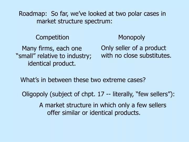
Roadmap: So far, we’ve looked at two polar cases in market structure spectrum:. Competition Monopoly. Only seller of a product with no close substitutes. Many firms, each one “small” relative to industry; identical product.

E N D
Roadmap: So far, we’ve looked at two polar cases in market structure spectrum: Competition Monopoly Only seller of a product with no close substitutes. Many firms, each one “small” relative to industry; identical product. What’s in between these two extreme cases? Oligopoly (subject of chpt. 17 -- literally, “few sellers”): A market structure in which only a few sellers offer similar or identical products.
In oligopoly: Firms are interdependent: Profits of my firm depend on my decisions (about price, output, etc.), but also on my rivals’ decisions. Interdependence gives rise to . . . Strategic behavior: As I decide what decision to make, I consider how my rivals might respond to my decision. (Note: Features not present in comp. or monopoly.)
Exmple: Identical product (widget) “duopoly” (2 firms). Market demand (in “inverse form”): P = 14 - 0.1 Q (Q = “industry” output = q1 + q2) Total cost of output for firm 1: TC(q1) = 2 q1 (Fixed costs are zero; marginal cost constant at $2/widget) Same cost function for firm 2.
($/widget) 14 Demand “Competitive” outcome 2 MC (widgets/day) 120 140 The efficient (“competitive”) outcome determined by P = MC. Pc = 2 $/widget. Qc = 120 widgets/day. Each duopolist produces 60 widgets/day. We get the competitive equilibrium when firms act like price takers. Not very likely in this case -- with only 2 firms, they’re likely to recognize their influence on price.
Another possibility: Maybe the 2 duopolists will cooperate -- behave like a single monopolist to maximize joint profit. Collusion: An agreement among firms in a market about quantities to produce or prices to charge. Cartel: A group of firms acting in unison. (Remember OPEC?)
The problem for the cartel: Pick joint output (Q) to maximize joint profit (joint ). One approach using a table: Q P TR TC joint 0 14 0 0 0 10 13 130 20 110 20 12 240 40 200 . . . . . (etc.) Joint max at Qm = 60 wdgts/day with Pm = 8 $/wdgt.
Another approach (for those who know some calculus): Joint profit as a function of Q (Q) = P x Q - 2 x Q = (14 - 0.1 Q) x Q - 2 x Q. = 12 Q – 0.1 Q2 Plotting this function with profit () on the vertical axis and output (Q) on the horizontal axis . . .
($/day) 360 Q (wdgts/day) 120 0 60 Solution: Qm = 60 widgets/day. Maximum joint profit = 360 $/day. To find max output, take the derivative of profit function . . . ’(Q) = 12 – 0.2 Q Set equal to zero and solve for Qm.
Each duopolist produces 30 widgets/day and earns: 1 = 2 = (8 x 30) - (2 x 30) = 180 $/day. To achieve this cartel (or “monopoly”) outcome, each duopolist has to observe a “quota;” . . . . . . that is, it has to limit its output to 30 wdgts/day. (Joint max requires restricting output relative to the competitive level.) Graphically . . .
($/widget) 14 Demand “Monopoly” outcome 8 “Competitive” outcome 2 MC (widgets/day) 60 120 140 MR Add “monopoly” MR “Monopoly” (cartel) outcome determined by MR = MC. Pm = 8 $/widget. Qm = 60 widgets/day. Not very likely either. Each duopolist has an incentive to produce more than its cartel (joint-profit-max) quota.
We’ve already seen: If both firms observe the cartel quota (q1 = q2 = 30): 1 = 2 = 180 $/day. Now suppose that firm 1 observes the quota (q1 = 30) but firm 2 “cheats,” producing q2 = 40. Then Q = 70 and P = 14 - 0.1 Q = 7 so: 1 = (30 x 7) - (30 x 2) = 150 $/day 2 = (40 x 7) - (40 x 2) = 200 $/day By “cheating” (producing more than its cartel quota), firm 2 gains at firm 1’s expense!
This illustrates interdependence: Firm 1’s profit changes with firm 2’s strategy. And it suggests a role for strategic behavior. (As I plan my strategy, I try to anticipate my rival’s reaction.) Firm 1’s reasoning: “Why should I be the sucker and stick to the quota knowing that firm 2 has incentive to over-produce.” “Come to think of it, even if firm 2 does stick to the quota, I’m better off if I cheat!”
Suppose both firms produce 40 (q1 = q2 = 40). Then Q = 80 and P = 14 - 0.1 Q = 6. 1 = 2 = (40 x 6) - (40 x 2) = 160 $/day. Claim: Given that q1 = 40, firm 2’s best output is q2 = 40. Given that q2 = 40, firm 1’s best output is q1 = 40. How could we verify this claim? Could set up a table showing firm 1’s profit for various values of q1, holding q2 fixed at 40.
Or, for those who know some calculus: Assuming q2 = 40, P = 14 - 0.1 x (q1 + 40), and . . . 1(q1) = [14 - 0.1 x (q1 + 40)] x q1 - 2 x q1 = 8 q1 – 0.1 q12 Maximize 1 with respect to q1: Solution q1 = 40. Symmetric problem for firm 2 yields q2 = 40 as profit-maximizing output level when q1 = 40.
This means that q1 = q2 = 40 is a “Nash equilibrium” . . . . . . named in honor of John Nash. http://abeautifulmind.com/
Nash, a mathematician, made contributions that are extremely valuable in modern economic theory. Jointly with two others (John Harsanyi and Reinhard Selten), he was awarded the 1994 Nobel Prize in Economics “for their pioneering analysis of equilibria in the theory of non-cooperative games.” http://nobelprize.org/economics/laureates/1994/ Nash was recognized for work that formed the basis for his Ph.D. dissertation in mathematics at Princeton.
Nash equilibrium pertains to situations (“games”) in which interdependent economic actors (“players”) face choices among strategies. Nash equilibrium: A set of strategies, one for each player, such that each player’s strategy is his/her best choice given the strategies chosen by the other players. (http://en.wikipedia.org/wiki/Nash_equilibrium) Again: Given q2 = 40, firm 1 gets max. profit with q1 = 40. Given q1 = 40, firm 2 gets max. profit with q2 = 40.
Nash equilibrium gives us a more realistic prediction of the outcome in our identical product duopoly. Unlike “competitive” outcome, it doesn’t rely on price-taking behavior (unrealistic with only 2 firms). Unlike “monopoly” outcome, it doesn’t assume that firms will adhere to a cartel quota even though they have individual incentives to cheat. In Nash equilibrium, neither firm has incentive to unilaterally change strategy.
($/widget) 14 Demand “Monopoly” outcome 8 Nash equilibrium outcome 6 “Competitive” outcome 2 MC (widgets/day) 60 80 120 140 Nash equilibrium outcome: PN = 6 QN = 80 (each duopolist produces 40) For this duopoly case, Nash equilibrium is “between” “monopoly” and “competitive” outcomes. This is true for oligopoly in general. As number of firms increases, Nash gets closer to “competitive.”