Download
1 / 53
540 likes | 797 Views
Viewing in 3D. Chapter 6. The 3D viewing process is inherently more complex than is the 2D viewing process. In 2D, we simply specify a window on the 2D world and a viewport on the 2D view surface.

E N D
Viewing in 3D Chapter 6
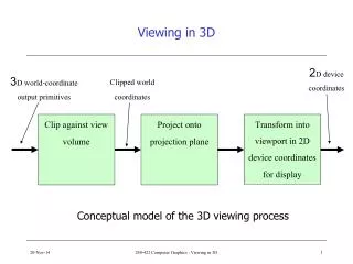
The 3D viewing process is inherently more complex than is the 2D viewing process. • In 2D, we simply specify a window on the 2D world and a viewport on the 2D view surface. • Conceptually, objects in the world are clipped against the window and then transformed into the viewport for display. • Although 3D viewing may seem overwhelming at first, it is less daunting when viewed as a series of easily understood steps, many of which we have prepared for in earlier chapters. Chapter 6 -- Viewing in 3D
1. The Synthetic Camera and Steps in 3D Viewing • A useful metaphor for creating 3D scenes is the notion of a synthetic camera Chapter 6 -- Viewing in 3D
While the synthetic camera is a useful concept, there is a bit more to producing an image than just pushing a button. • Creation of our photo is accomplished as a series of steps: • Specification of projection type • Specification of viewing parameters • Clipping in three dimensions • Projection and Display Chapter 6 -- Viewing in 3D
2. Projections • In general, projections transform points in a coordinate system of dimension n into points in a coordinate system of dimension less than n. • For now we shall limit ourselves to 3D to 2D. Chapter 6 -- Viewing in 3D
The projection of a 3D object is defined by straight projection rays, called projectors, emanating from a center of projection, passing through each point of the object, and intersecting a projection plane to form the projection. • Two locations for the center of projection: • finite distance (perspective projection) and • infinite distance (parallel projection) Chapter 6 -- Viewing in 3D
2.1 Perspective Projections • The perspective projections of any set of parallel lines that are not parallel to the projection plane converge to a vanishing point. • if the set of lines is parallel to one of the three principal axes, the vanishing point is called an axes vanishing point Chapter 6 -- Viewing in 3D
Perspective projections are categorized by their number of principal vanishing points • One point perspective projection Chapter 6 -- Viewing in 3D
Two point perspective projection Chapter 6 -- Viewing in 3D
2.2 Parallel Projections • Parallel projections are categorized into two types, depending on the relation between the direction of projection and the normal to the projection plane. • The two most common are: • orthographic -- direction of the projection and the normal of the plane are the same • oblique -- they are not the same. Chapter 6 -- Viewing in 3D
The most common types of orthographic projections are • front-elevation • top-elevation • side-elevation Chapter 6 -- Viewing in 3D
A special sub-type of orthographic projections are isometric projections. The projection plan normal makes equal angles with each principal axis. Chapter 6 -- Viewing in 3D
The other type of parallel projection is an Oblique projection • the projection plane normal and the direction of the projection differ. Chapter 6 -- Viewing in 3D
3. Specification of an Arbitrary 3D View • 3D viewing involves not just a projection, but also a view volume against which the 3D world is clipped. • The projection and the view volume together provide all the information that we need to clip and project into 2D space. • Then the 2D transformation into physical device coordinates is straightforward. Chapter 6 -- Viewing in 3D
The projection plane (view plane in the graphics literature) is defined by • a point in the plane called a view reference point (VRP) and • a normal to the plane called the view-plane normal (VPN) Chapter 6 -- Viewing in 3D
To define a window on the view plane, we need to specify minimum and maximum window coordinates Chapter 6 -- Viewing in 3D
for a perspective projection it looks like: for a parallel projection it looks like: • The center of projection and direction of projection are defined by the Projection Reference Point (PRP) Chapter 6 -- Viewing in 3D
At times we may want the view volume to be finite, in order to limit the number of output primitives projected onto the view plane. • You specify the front and back clipping planes • For parallel projections it looks like: • for perspective projections it looks like: Chapter 6 -- Viewing in 3D
4. Examples of 3D Viewing • In this section, we consider how we can apply the basic viewing concepts introduced in Section 3 to create a variety of projections. • such as this house. Chapter 6 -- Viewing in 3D
Because this house is used throughout this section, it will be helpful to remember its dimensions and position, which are indicated here: Chapter 6 -- Viewing in 3D
4.1 Perspective Projections • To obtain the front one-point perspective view shown here: • position the center of projection (the viewer) at (8,6,84) Chapter 6 -- Viewing in 3D
To make the vie larger and centered, • make the view plane and the front of the house coincide. • place the viewer at (8, 6, 30) in front of this plane. Chapter 6 -- Viewing in 3D
Other views could look like: Chapter 6 -- Viewing in 3D
And Chapter 6 -- Viewing in 3D
4.2 Parallel Projections Chapter 6 -- Viewing in 3D
4.3 Finite View Volumes • In all the examples so far, the view volume has been assumed to be infinite. • If we start with this setup Chapter 6 -- Viewing in 3D
and add a far clipping plane right in front of the far wall of the house, we can end up with an image that looks like: Chapter 6 -- Viewing in 3D
5. The Mathematics of Planar Geometric Projections • Here we introduce the basic mathematics of planar geometric projections. • For simplicity, we start by assuming that, • in the perspective projection, the projection plane is normal to the z axis at z=d, • and that in the parallel projection, the projection plane is at z=0. Chapter 6 -- Viewing in 3D
Each of the projections can be defined by a 4x4 matrix. • This is convenient, because the projection matrix can be composed with the transformation matrices, allowing two operations (transform then project) to be represented in a single matrix. • In this section we derive 4x4 matrices for several projections Chapter 6 -- Viewing in 3D
Given a point P to be projected onto the plane, calculate the point Pp=(xp, yp, zp) which is the projection. We use similar triangles as found in this figure and calculate ratios for the transformation as: Chapter 6 -- Viewing in 3D
These ratios lead to a transformation matrix for a perspective projection of: Chapter 6 -- Viewing in 3D
The orthographic projection pane at z=0 is straightforward, and ends up as: Chapter 6 -- Viewing in 3D
6. Implementation of Planar Geometric Projections • Given a view volume and a projection, let us consider how the viewing operation of clipping and projecting is applied. • The brute force method was: • clip each line with the 6 planes of the volume. • project remaining lines by solving simultaneous equations for the projection onto the view plane • Then transform these to 2D space... Chapter 6 -- Viewing in 3D
The large number of calculations required for this process, repeated for many lines, involves considerable computing. • Happily there is a more efficient procedure, based on the divide-and-conquer strategy of breaking down a difficult problem into a series of simpler ones. • And they are much easier if you use the canonical volumes shown here: Chapter 6 -- Viewing in 3D
Our goal is to find the normalizing transformations Npar and Nper that transform an arbitrary parallel or perspective projection view volume into the parallel and perspective view volumes • Then the rest of the process is done • clipping, • projection into 2D Chapter 6 -- Viewing in 3D
6.1 The Parallel Projection Case • In this section, we derive the normalizing transformation Npar for parallel projections. • This is done in order to transform world-coordinate positions such that the view volume is transformed into the canonical view volume. • Then we clip and project. Chapter 6 -- Viewing in 3D
Transformation Npar is derived for the most general case, the oblique (rather than the orthographic) parallel projection. • Npar thus includes a shear transformation that causes the direction of projection in viewing coordinates to be parallel to z. • By including this shear we can do the projection onto z=0 plane simply by setting z=0. Chapter 6 -- Viewing in 3D
The series of transformations that make up Npar is as follows: • Translate the VRP to the origin • Rotate VRC such that the n axis (VPN) becomes the z axis, the u axis becomes the x axis, and the v axis becomes the y axis. • Shear such that the direction of projection becomes parallel to the z axis. • Translate and scale into the parallel-projection canonical view volume. Chapter 6 -- Viewing in 3D
6.2 The Perspective Projection Case • We now develop the normalizing transformation Nper for perspective projections. • Nper transforms world-coordinate positions such that the view volume becomes the perspective-projection canonical view volume, the truncated pyramid with the apex at the origin. • Then you clip and project using Mper derived in section 6.5. Chapter 6 -- Viewing in 3D
The series of transformations making up Nper as follows: • Translate VRP to the origin • Rotate VRC such that the n axis (VPN) becomes the z axis, the u axis becomes the x axis, and the v axis becomes the y axis. • Translate such that the center of projection (COP), given by the PRP, is at the origin. • Shear that the center line of the view volume becomes the z axis • Scale such that the view volume becomes the canonical perspective view volume, the truncated right pyramid. Chapter 6 -- Viewing in 3D
This figure presents the view volume before and after the steps just described. Chapter 6 -- Viewing in 3D
6.3 Clipping Against a Canonical View Volume in 3D • The canonical view volumes are: • the 2x2x1 prism for parallel projections • the truncated right regular pyramid for perspective projections Chapter 6 -- Viewing in 3D
Both the Cohen-Sutherland and Cyrus-Beck clipping algorithms discussed in Chapter 3 readily extend to 3D • There are also other clipping algorithms that are based on parametric expressions that can be more efficient than the simple Cohen-Sutherland algorithm (see Chapters 6 and 19 of Foley, vanDam, et.al. --the big white book). Chapter 6 -- Viewing in 3D
6.4 Clipping in Homogeneous Coordinates • There are two reasons to clip in homogeneous coordinates: • efficiency • translate perspective canonical to parallel canonical and do a single clip -- Hardware does this. • if you get a point with negative W it can be clipped in homogeneous, but not in 3D • get negative W’s from unusual homogeneous transformations and from the use of parametric splines. Chapter 6 -- Viewing in 3D
With regard to clipping, it can be shown that the transformation from the perspective-projection canonical view volume to the parallel-projection canonical view volume is: Chapter 6 -- Viewing in 3D
This matrix translates the canonical view volumes as shown: • As we will see in Chapter 9, it is sometimes desirable to represent points directly in homogeneous coordinates with arbitrary W. Chapter 6 -- Viewing in 3D
6.5 Mapping into a Viewport • Output primitives are clipped in the normalized projection coordinate system, which is also called the 3D screen coordinate system Chapter 6 -- Viewing in 3D
6.6 Implementation Summary • There are two generally used implementations of the overall viewing transformation • The first was discussed in Sections 6.6.1 through 6.6.3 • appropriate when primitives are defined in 3D and the transformations never create a negative W. • The second was discussed in Section 6.6.4 • required whenever primitives are defined and might have W<0, when transformations might create a W<0, or a single clip algorithm is implemented. Chapter 6 -- Viewing in 3D
7. Coordinate Systems • Several different coordinate systems have been used in Chapters 5 and 6. • In this section we summarize all the systems, and also discuss their relationships to one another. Chapter 6 -- Viewing in 3D