3D Viewing III

1. 3D Viewing III

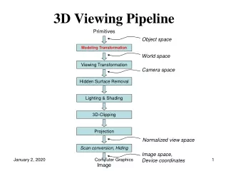
2. Viewing in Three DimensionsMathematics of Projections • Lecture roadmap • mathematics of planar geometric projections • how to get from view specification to 2D image? • deriving 2D image from 3D view parameters is a hard problem • easier to take a picture from • canonical view volume (3D parallel projection cuboid) • canonical view position (camera at the origin, looking down the negative z-axis) • break into three stages: • get parameters for view specification (covered in last lecture) • transform from specified view volume into canonical view volume • using canonical view, clip, project, and rasterize scene to make 2D image

3. Stage One: Specifying a View Volume • Reduce degrees of freedom; four steps to specifying view volume • Position camera (and therefore its view/film plane) • Orient camera to point at what you want to see • Define field of view perspective: aspect ratio of film and angle of view: between wide angle, normal, and zoom parallel: width and height 4. Choose perspective or parallel projection (Optional: Specify a focal distance and exposure time. Our camera won’t do this.)

4. Examples of a View Volume (1/2) • Perspective Projection: Truncated Pyramid – Frustum • Look vector is the center line of the pyramid, the vector that lines up with “the barrel of the lens” Width Look Height Near

5. y Width Far distance x z Height Look vector Near distance Up vector Position Examples of a View Volume (2/2) • Orthographic Parallel Projection: Truncated View Volume – Cuboid • Orthographic parallel projection has no view angle parameter

6. Specifying Arbitrary 3D Views • Placement of view volume (visible part of world) specified by camera’s position and orientation • Position (a point) • Look and Upvectors • Shape of view volume specified by • horizontal and vertical view angles • front and back clipping planes • Perspective projection: projectors intersect at Position • Parallel projection: projectors parallel to Look vector, but never intersect (or intersect at infinity) • Coordinate Systems • world coordinates– standard right-handed xyz 3-space • camera coordinates– camera-space right handed coordinate system (u, v, w); origin at Position and axes rotated by orientation; used for transforming arbitrary view into canonical view position Perspective projection Look vector Parallelprojection Image Source: Steve Marschner, Cornell ‡ ‡ v isn't strictly the Up vector but the projection of Up

7. Up • parallel projection • sits at origin: • Position = (0, 0, 0) • looks along negative z-axis: • Look vector = (0, 0, –1) • oriented upright: • Up vector = (0, 1, 0) • film plane extending from –1 to 1 in x and y z Look Up Arbitrary View VolumeToo Complex • We have specified arbitrary view with viewing parameters • Problem: map arbitrary view specification to 2D image of scene. This is hard, both for clipping and for projection • Solution: reduce to a simpler problem and solve • Note: Look vector along negative, not positive, z-axis is arbitrary but makes math easier; ditto choosing • there is a view specification from which it is easy to take a picture. We’ll call it the canonical view: from the origin, looking down the negative z-axis – think of the scene as lying behind a window and we’re looking through that window

8. Stage 2: Normalizing to the Canonical View Volume • Goal: transform arbitrary view and world to canonical view volume, maintaining relationship between view volume and world, then take picture • for parallel view volume, transformation is affine†: made up of linear transformations (rotations and scales) and translation/shift • in case of a perspective view volume, it also contains a non-affine perspective transformation that turns a frustum into a parallel view volume, a cuboid • composite transformation to transform arbitrary view volume to canonical view volume, named the normalizing transformation, is still a 4x4 homogeneous matrix that typically has an inverse • easy to clip against this canonical view volume; clipping planes are axis-aligned! • projection using canonical view volume is even easier: just omit z-coordinate • for oblique parallel projection, a shearing transform is part of composite transform, to “de-oblique” view volume † Affine transformations preserve parallelism but not lengths and angles. The perspective transformation is a type of non-affine transformation known as a projective transformation, which does not preserve parallelism

9. Viewing Transformation Normalizing Transformation • Problem of “taking a picture” has now been reduced to problem of finding correct normalizing transformation • Finding rotation component of normalizing transformation is hard. • Easier to find inverse of rotational component (as you will see in a few slides.) • Digression: • find inverse of normalizing transformation • called the viewing transformation • turns the canonical view into the arbitrary view • (x, y, z) to (u, v, w)

10. Building Viewing Transformation from View Specification • We know the view specification: Position, Look vector, and Up vector • Need to derive an affine transformation from these parameters to translate and rotate the canonical view into our arbitrary view • the scaling of the film (i.e. the cross-section of the view volume) to make a square cross-section will happen at a later stage, as will clipping • Translation is easy to find: we want to translate the origin to the point Position; therefore, the translation matrix is • Rotation is harder: how do we generate a rotation matrix from the viewing specifications to turn x, y, z, into u, v, w? • a digression on rotation will help answer this

11. Rotation (1/4) 3 x 3 rotation matrices • We learned about 3 x 3 matrices that “rigid-body rotate” the world (we’re leaving out the homogeneous coordinate for simplicity) • When they do, the three unit vectors that used to point along the x, y, and z axes are rotated to a new orientation • Because it is a rigid-body rotation • resulting vectors are still unit length • resulting vectors are still perpendicular to each other • resulting vectors still satisfy the “right hand rule” • Any matrix transformation with these three properties is a rotation about some axis by some amount! • Let’s call the three x-axis, y-axis, and z-axis-aligned unit vectors e1, e2, e3 • Writing out:

12. Rotation (2/4) • Let’s call our rotation matrix M, and let’s label its columns v1, v2, and v3: • When we multiply M by e1, what do we get? • Similarly for e2 and e3: • Therefore M = [u v w] where u, v, and w are unit column vectors, will rotate the x, y, z axes into the u, v, w axes • And M-1would rotate the u, v, w axes into the x, y, z axes, which is what we actually want... • Therefore we first find M by computing u, v and w from the viewing specification parameters, and then we need to find an easy way of getting the inverse of M. is the third column of M is the first column of M is the second column of M

13. vi •vi=1 because ||vi|| = 1 but all other vi • vj = 0 (ij) Rotation (3/4) • First, solve easier problem of finding the inverse of a rotation matrix • As we learned in the transformations lecture, for a rotation matrix with columns vi • columns must be unit vectors: ||vi|| = 1 • columns are perpendicular: vi•vj = 0 (ij) • Therefore • We can write this matrix dot products as where MT is a matrix whose rows are v1, v2, and v3 • Also, for matrices in general, M-1M = I, (actually, M-1 exists only for “well-behaved” matrices) • Therefore, for rotation matrices, we have just shown that M-1 is simply MT • MT is trivial to compute, M-1 takes considerablework: big win!

14. Rotation (4/4) Summary • If M is a rotation matrix, then its columns are pairwise perpendicular and have unit length • Inversely, if the columns of a matrix are pairwise perpendicular and have unit length, then the matrix is a rotation • For such a matrix, • Most importantly, then and this will help us build the normalizing transformation from the easier to find viewing transformation.

15. Building the Orientation Matrix • Know how to invert a rotation matrix, but how do we build it from the viewing specification to to normalize the camera-space unit vector axes (u, v, w) located at the origin into the world-space axes (x, y, z). • rotation matrix M will turn (x, y, z) into (u, v, w) and has columns (u, v, w) - viewing matrix • conversely, M-1=MTturns (u, v, w) into (x, y, z). MT has rows (u, v, w)-normalization matrix • Reduces the problem of finding the correct rotation matrix into finding the correct perpendicular unit vectors u, v, and w • Restatement of rotation problem: Using Position, Look vector, and Up vector, compute viewing rotation matrix M with columnsu, v, and w, then use its inverse, the transpose MT, with row vectors u, v, w to get the normalization rotation matrix

16. y x z v v Projection of Up Up Look u u w w Finding u, v, and w from Position, Look, and Up (1/6) Look • We know that we want the (u, v, w) axes to have the following properties: • our arbitrary Look Vector will lie along the negative w-axis • a projection of the Up Vector into the plane defined by the w-axis as its normal will lie along the v-axis • The u-axis will be mutually perpendicular to the v and w-axes, and will form a right-handed coordinate system • Plan of attack: first find w from Look, then find v from the Up and w vector, then find u as a normal to the plane defined by w and v -z Up Plane defined by w axis w

17. y x z -z v Up Look u w Finding u, v, and w (2/6) Finding w • Finding w is easy. Look vector in canonical volume lies on –z. Since z maps to w, w is a normalized vector pointing in the opposite direction from our arbitrary Look vector • Note that Up and w define a plane, and that u is a normal to that plane, and that v is anormal to the plane defined by w and u -z

18. y x z v Up u Look w Finding u, v, and w (3/6) Finding v • Problem: find a vector, v, perpendicular to w • Solution: project out the w component of the Up vector and normalize -z • w is unit length, but Up vector might not be unit length or perpendicular to w, so we have to remove the w component and then normalize • By removing the w component from the Up vector, the resulting vector is the component of Up in a direction perpendicular to w • To create the orthogonal coordinate frame of the camera we need a third vector

19. y x z v Up u Look w Finding u, v, and w (4/6) Finding u • We can use cross-product, but which one should we use? • w X v and v X w are both perpendicular to the plane, but in different directions . . . • Answer: cross-products are right-handed, so use v X w to create a right-handed coordinate frame • As a reminder, the cross product of two vectors a and b is: -z

20. y x z -z v Up u Look w Finding u, v, and w (6/6) To summarize • The viewing transformation is now fully specified • knowing u, v, and w, we can rotate the canonical view into the user-specified orientation • we already know how to translate the view • Important Note: we don’t actually apply the forward viewing transformation. Instead, the inverse viewing transformation, namely the normalizing transformation, will be used to map the arbitrary view into the canonical view

21. Transforming to the Canonical View The Viewing Problem for Parallel Projection • Given a parallel view specification and vertices of a bunch of objects, we use the normalizing transformation, i.e., the inverse viewing transformation, to normalize the view volume to a cuboid at the origin, then clip, and then project those vertices by ignoring their z values The Viewing Problem for Perspective Projection • Normalize the perspective view specification to a unit frustum at the origin looking down the –z axis; then transform the perspective view volume into a parallel (cuboid) view volume, simplifying both clipping and projection Note: it’s a cuboid, not a cube (transformation arithmetic and clipping are easier)

22. Normalizing the View Volume The Parallel Case • Decomposes into multiple steps • Each step defined by a matrix transformation • The product of these matrices defines the whole transformation in one large, composite matrix. The steps are: • move the eye/camera to the origin • transform the view so that (u, v, w) is aligned with (x, y, z) • adjust the scales so that the view volume fits between –1 and 1 in x and y, the back clip plane lies at z = –1, the front plane at z = 0 The Perspective Case • Same as parallel, but add one more step: • distort pyramid to cuboid to achieve perspective distortion to align the front clip plane with z = 0

23. Normalizing the View Volume Step 1 Move the eye to the origin • We want a matrix to transform (Posx,Posy,Posz) to (0, 0, 0) • Solution: it’s just the inverse of the viewing translation transformation: (tx, ty, tz) = (–Posx, –Posy, –Posz) • We will take the matrix: and we will multiply all vertices explicitly (and the camera implicitly) to preserve the relationship between camera and scene, i.e., for all vertices p • This will move Position (the “eye point”) to (0, 0, 0)

24. Normalizing the View Volume Step 2 • Position now at origin But we’re hardly done! Still need to: • align orientation with x,y,z world coordinate system • normalize proportions of the view volume y Look z x

25. Normalizing the View Volume Step 3 Rotate the view and align with the world coordinate system • We found out that the view transformation matrix M with columns u, v, and w would rotate the x, y, z axes into the u, v, and w axes • We now apply the inverse (transpose) of that rotation, MT, to the scene. That is, a matrix with rowsu, v, and w will rotate the axes u, v, and w into the axes x, y, and z • Define Mrot to be this rotation matrix transpose • Now every vertex in the scene (and the camera implicitly) is multiplied by the composite matrix We’ve translated and rotated, so that the Position is at the origin, and the (u, v, w) axes and the (x, y, z) axes are aligned current situation Look

26. y y z z x x Normalizing the View Volume Step 4 • We’ve gotten things more or less to the right place, but the proportions of the view volume need to be normalized… • last affine transformation: scaling • Need to be normalized to a square cross-section 2-by-2 units • why is that preferable to the unit square? • Adjust so that the corners of far clipping plane eventually lie at (+1,+1, –1) • One mathematical operation works for both parallel and perspective view volumes • Imagine vectors emanating from origin passing through corners of far clipping plane. For perspective view volume, these are edges of volume. For parallel, these lie inside view volume • First step: force vectors into 45-degree angles with x and y axes • We’ll do this by scaling in x and y

27. Normalizing the View Volume Step 5 Scaling Clipping Planes • Scale independently in x and y:looking down from above, we see this: • Want to scale in x to make angle 90 degrees • Need to scale in x by • Similarly in y

28. Normalizing the View Volume Step 6 The xy scaling matrix • The scale matrix we need looks like this: • So our current composite transformation looks like this: The xy scaling matrix

29. Normalizing the View Volume Step 7 One more scaling matrix • Relative proportions of view volume planes are now correct, but the back clipping plane is probably lying at some z –1, and we want all points inside view volume to have 0 ≤ z ≤ -1 • Need to shrink the back (far) plane to be at z = –1 • The z distance from the eye to that point has not changed: it’s still far (distance to far clipping plane) • If we scale in z only, proportions of volume will change; instead we scale uniformly:

30. y (-1,1,-1) (-k,k,-k) z z = -1 x Normalizing the View Volume Step 8 • The Current Situation • Far plane at z = –1. • Near clip plane now at z = –k (note k > 0)

31. The Results • Our near-final composite normalizing transformation for canonical perspective view volume: • Ttrans takes the camera’s Position and moves the camera to the world origin • Mrot takes the Look and Up vectors and orients the camera to look down the –z axis • Sxy takes and scales the clipping planes so that the corners are at (±1, ±1) • Sfar takes the far clipping plane and scales it to lie on the z=-1 plane

32. The Perspective Transformation (1/5) • We’ve put the perspective view volume into canonical position, orientation and size • Let’s look at a particular point on the original near clipping plane lying on the Look vector: It gets moved to a new location on the negative z-axis, say

33. The Perspective Transformation (2/5) • What is the value of k? Trace through the steps. p first gets moved to just • This point is then rotated to (near)(–e3) • The xy scaling has no effect, and the far scaling changes this to , so

34. The Perspective Transformation (3/5) • Transform points in standard perspective view volume between –k and –1 to standard parallel view volume • “z-buffer,” used for visible surface calculation, needs z values to be [0 1], not [–1 0]. Perspective transformation must therefore transform scene to positive range 0 ≤ z ≤ 1 • The matrix that does this: • (Remember that 0< k < 1 …) • Why not originally align camera to +z axis? • Choice is perceptual, we think of looking through a display device into the scene that lies behind window Note: not 1! Flip the z-axis and unhinge

35. k+d k+d k+d k+d w k+d k+d The Perspective Transformation (4/5) • Take a typical point prior to perspective transform p= and rewrite it as • ; p is parameterized by distance along frustum • when d = 0, p is on near clip plane; when d = (1-k), p is on far clip plane • depending on x, y, and z, p may or may not actually fall within frustum • Apply D (from previous slide) to p to get new point p’ • Note: so in the last step we must divide through by !!! • this causes x and y to be “perspectivized”, with points closer to the near clip plane being scaled up the most • this also transforms z, but z is tossed out when we project onto the film plane so it ultimately doesn’t matter • understanding homogenous coordinates is essential to graphics • Try values of d: 0, 1-k, ½(1-k), -1, 1

36. k+d k+d k+d The Perspective Transformation (5/5) • Again consider • What happens to x and y when d gets very large? • note: when we let d increase beyond (1-k), p is now beyond the frustum (such lines will be clipped) • This result provides perspective foreshortening: parallel lines converge to a vanishing point • What happens when d is negative? • now p lies in front of the near clip plane, possibly behind the eye point • result: when becomes negative, the signs of x and y will be flipped: text would be upside-down and backwards • you won’t see these points because they are clipped • What happens after perspective transformation? • Answer: parallel projection is applied to determine location of points onto the film plane • projection is easy: drop z! • however, we still need to keep the z ordering intact for visible surface determination (k+d)

37. The End Result • Final transformation: • Note that once the viewing parameters (Position, Up vector, Look vector, Height angle, Aspect ratio, Near, and Far) are known, the matrices can all be computed and multiplied together to get a single 4x4 matrix that is applied to all points of all objects to get them from “world space” to the standard parallel view volume. • This is a huge win for homogeneous coordinates • NOTE: Slide nomenclature differs from the book: • k is –c in the book • near is n, far is f

38. Stage 3: Making 2D Image • So far we’ve • Specified the view volume • Transformed from the specified view volume into the canonical view volume • Last stage involves • Clipping • Projecting

39. (-1, 1, 1) (-1, 1, 0) y (1, 1, 1) (1, 1, 0) z (-1, -1, 0) (-1, -1, 1) x Front clip plane transforms to here (1, -1, 1) Back clip plane transforms to the z=1 plane (1, -1, 0) Clipping • We said that taking the picture from the canonical view would be easy: final steps are clipping and projecting onto the film plane • Need to clip scene against sides of view volume • However, we’ve normalized our view volume into an axis-aligned cuboid that extends from –1 to 1 in x and y and from 0 to 1 in z • Note: This is the flipped (in z) version of the canonical view volume • Clipping is easy! Test x and y components of vertices against +/-1. Test z components against 0 and 1

40. Clipping (cont.) • Vertices falling within these values are saved, and vertices falling outside get clipped; edges get clipped by knowing x,y or z value at an intersection plane. Substitute x, y, or z = 1 in the corresponding parametric line equations to solve for t • In 2D: (x1, y1, z1 ) t=1 t=0 (x0, y0, z0 ) y (1, 1) (x1, y1 ) x=1 x (x0, y0 ) (-1, -1)

41. Projection • Can make an image by taking each point and “ignoring z” to project it onto the xy-plane • A point (x,y,z) where turns into the point (x’, y’) in screen space (assuming viewport is the entire screen) with by - ignoring z - - • If viewport is inside a Window Manager’s window, then we need to scale down and translate to produce “window coordinates” • Note: because it’s a parallel projection we could have projected onto the front plane, the back plane, or any intermediate plane … the final pixmap would have been the same 1. Note that these functions are not exactly correct since if x or y is ever 1, then we will get x’ or y’ to be 1024 which is out of our range, so we need to make sure that we handle these cases gracefully. In most cases, making sure that we get the floor of 512(x+1) will address this problem since the desired x will be less than 1.

42. Summary • Entire problem can be reduced to a composite matrix multiplication of vertices, clipping, and a final matrix multiplication to produce screen coordinates. • Final composite matrix (CTM) is composite of all modeling (instance) transformations (CMTM) accumulated during scene graph traversal from root to leaf, composited with the final composite normalizing transformation N applied to the root/world coordinate system: • Preview of Applications: • 1) You will be computing the normalizing transformation matrix N in Camtrans • 2) In Sceneview, you will extend your Camera with the ability to traverse and compute composite modeling transformations (CMTMs) to produce a single CTM for each primitive in your scene. 1) 2) for every vertex P defined in its own coordinate system 3) 4) for all clippedP’