Download
1 / 108
1.13k likes | 2.2k Views
CMOS Active Filters. G ábor C. Temes School of Electrical Engineering and Computer Science Oregon State University Rev. Sept. 2011. Structure of the Lecture. Continuous-time CMOS filters; Discrete-time switched-capacitor filters (SCFs); Non-ideal effects in SCFs;

E N D
CMOS Active Filters Gábor C. Temes School of Electrical Engineering and Computer Science Oregon State University Rev. Sept. 2011
Structure of the Lecture • Continuous-time CMOS filters; • Discrete-time switched-capacitor filters (SCFs); • Non-ideal effects in SCFs; • Design examples: a Gm-C filter and an SCF; • The switched-R/MOSFET-C filter.
Classification of Filters • Digital filter: both time and amplitude are quantized. • Analog filter: time may be continuous (CT) or discrete (DT); the amplitude is always continuous (CA). • Examples of CT/CA filters: active-RC filter, Gm-C filter. • Examples of DT/CA filters: switched-capacitor filter (SCF), switched-current filter (SIF). • Digital filters need complex circuitry, data converters. • CT analog filters are fast, not very linear and accurate, may need tuning circuit for controlled response. • DT/CA filters are linear, accurate, slower.
Filter Design • Steps in design: 1. Approximation – translates the specifications into a realizable rational function of s (for CT filters) or z (for DT filters). May use MATLAB to obtain Chebyshev, Bessel, etc. response. 2. System-level (high-level)implementation – may use Simulink, etc. Architectural and circuit design should include scaling for impedance level and signal swing. 3. Transistor-level implementation – may use SPICE, Spectre, etc. This lecture will focus on Step. 2 for CMOS filters.
Mixed-Mode Electronic System • Analog filters needed to suppress out-of-band noise and prevent aliasing. Also used as channel filters, as loop filters in PLLs and oversampled ADCs, etc. • In a mixed-mode system, continuous-time filter allows sampling by discrete-time switched-capacitor filter (SCF). The SCF performs sharper filtering; DSP filtering may be even sharper. • In Sit.1, SCF works as a DT filter; in Sit.2 it is a CT one.
Frequency Range of Analog Filters • Discrete active-RC filters: 1 Hz – 100 MHz • On-chip continuous-time active filters: 10 Hz - 1 GHz • Switched-capacitor or switched-current filters: 1 Hz – 10 MHz • Discrete LC: 10 Hz - 1 GHz • Distributed: 100 MHz – 100 GHz
Accuracy Considerations • The absolute accuracy of on-chip analog components is poor (10% - 50%). The matching accuracy of like elements can be much better with careful layout. • In untuned analog integrated circuits, on-chip Rs can be matched to each other typically within a few %, Cs within 0.05%, with careful layout. The transconductance (Gm) of stages can be matched to about 10 - 30%. • In an active-RC filter, the time constant Tc is determined by RC products, accurate to only 20 – 50%. In a Gm-C filter , Tc ~ C/Gm, also inaccurate. Tuning may be used. • In an SC filter, Tc ~ (C1/C2)/fc, where fc is the clock frequency. Tc accuracy may be 0.05% or better!
Design Strategies • Three basic approaches to analog filter design: 1. For simple filters (e.g., anti-aliasing or smoothing filters), a single-opamp stage may be used. 2. For more demanding tasks, cascade design is often used– split the transfer function H(s) or H(z) into first and second-order realizable factors, realize each by buffered filter sections, connected in cascade. Simple design and implementation, medium sensitivity and noise. 3. Multi-feedback (simulated reactance filter) design. Complex design and structure, lower noise and sensitivity. Hard to lay out and debug.
Active-RC Filters [1], [4], [5] • Single-amplifier filters: Sallen-Key filter; Kerwin filter; Rauch filter, Deliyannis-Friend filter. Simple structures, but with high sensitivity for high-Q response. • Integrator-based filter sections: Tow-Thomas biquads; Ackerberg-Mossberg filter. 2 or 3 op-amps, lower sensitivity for high-Q. May be cascaded. • Cascade design issues: pole-zero pairing, section ordering, dynamic range optimization. OK passband sensitivities, good stopband rejection. • Simulated LC filters: gyrator-based and integrator-based filters; dynamic range optimization. Low passband sensitivities and noise, but high stopband sensitivity and complexity in design, layout, testing.
Sallen-Key Filter [1],[4] First single-opamp biquad. General diagram: Often, K = 1. Has 5 parameters, only 3 specified values. Scaling or noise reduction possible. • Amplifier not grounded. Input common-mode changes with output. Differential implementation difficult.
Sallen-Key Filter • Transfer function: • Second-order transfer function (biquad) if two of the admittances are capacitive. Complex poles are achieved by subtraction of term containing K. • 3 specified parameters (1 numerator coefficient, 2 denominator coeffs for single-element branches).
Sallen-Key Filter • Low-pass S-K filter (R1, C2, R3, C4): • Highpass S-K filter (C1, R2, C3, R4): • Bandpass S-K filter ( R1, C2, C3, R4 or C1, R2, R3, C4):
Sallen-Key Filter • Pole frequency ωo: absolute value of natural mode; • Pole Q: ωo/2|real part of pole|. Determines the stability, sensitivity, and noise gain. Q > 5 is dangerous, Q > 10 can be lethal! For S-K filter, dQ/Q ~ (3Q –1) dK/K .So, if Q = 10, 1% error in K results in 30% error in Q. • Pole Q tends to be high in band-pass filters, so S-K may not be suitable for those. • Usually, only the peak gain, the Q and the pole frequency ωo are specified. There are 2 extra degrees of freedom. May be used for specified R noise, minimum total C, equal capacitors, or K = 1. • Use a differential difference amplifier for differential circuitry.
Kerwin Filter • Sallen-Key filters cannot realize finite imaginary zeros, needed for elliptic or inverse Chebyshev response. Kerwin filter can, with Y = G or sC. For Y = G, highpass response; for Y = sC, lowpass.
Deliyannis-Friend Filter [1] Single-opamp bandpass filter: • Grounded opamp, Vcm = 0. The circuit may be realized in a fully differential form suitable for noise cancellation. Input CM is held at analog ground. • Finite gain slightly reduces gain factor and Q. Sensitivity is not too high even for high Q.
Deliyannis-Friend Filterα • Q may be enhanced using positive feedback: • New Q = • α = K/(1-K) • Opamp no longer grounded, Vcm not zero, no easy fully differential realization.
Rauch Filter [1] Often applied as anti-aliasing low-pass filter: Transfer function: • Grounded opamp, may be realized fully differentially. 5 parameters, 3 constraints. Min. noise, or C1 = C2, or min. total C can be achieved.
Tow-Thomas Biquad [1] • Multi-opamp integrator-based biquads: lower sensitivities, better stability, and more versatile use. • They can be realized in fully differential form. • The Tow-Thomas biquad is a sine-wave oscillator, stabilized by one or more additional element (R1): • In its differential form, the inverter is not required.
Tow-Thomas Biquad • The transfer functions to the opamp outputs are Other forms of damping are also possible. Preferable to damp the second stage, or (for high Q) to use a damping C across the feedback resistor. Zeros can be added by feed-forward input branches.
Ackerberg–Mossberg Filter [1] • Similar to the Tow-Thomas biquad, but less sensitive to finite opamp gain effects. • The inverter is not needed for fully differential realization. Then it becomes the Tow-Thomas structure.
Cascade Filter Design [3], [5] • Higher-order filter can constructed by cascading low-order ones. The Hi(s) are multiplied, provided the stage outputs are buffered. • The Hi(s) can be obtained from the overall H(s) by factoring the numerator and denominator, and assigning conjugate zeros and poles to each biquad. • Sharp peaks and dips in |H(f)| cause noise spurs in the output. So, dominant poles should be paired with the nearest zeros.
Cascade Filter Design [5] • Ordering of sections in a cascade filter dictated by low noise and overload avoidance. Some rules of thumb: • High-Q sections should be in the middle; • First sections should be low-pass or band-pass, to suppress incoming high-frequency noise; • All-pass sections should be near the input; • Last stages should be high-pass or band-pass to avoid output dc offset.
Dynamic Range Optimization [3] • Scaling for dynamic range optimization is very important in multi-op-amp filters. • Active-RC structure: • Op-amp output swing must remain in linear range, but should be made large, as this reduces the noise gain from the stage output to the filter output. However, it reduces the feedback factor and hence increases the settling time.
Dynamic Range Optimization • Multiplying all impedances connected to the opamp output by k, the output voltage Vout becomesk.Vout, and all output currents remain unchanged. • Choose k.Vout so that the maximum swing occupies a large portion of the linear range of the opamp. • Find the maximum swing in the time domain by plotting the histogram of Vout for a typical input, or in the frequency domain by sweeping the frequency of an input sine-wave to the filter, and compare Vout with the maximum swing of the output opamp.
Impedance Level Scaling • Lower impedance -> lower noise, but more bias power! • All admittances connected to the input node of the opamp may be multiplied by a convenient scale factor without changing the output voltage or output currents. This may be used, e.g., to minimize the area of capacitors. • Impedance scaling should be done after dynamic range scaling, since it doesn’t affect the dynamic range.
Tunable Active-RC Filters [2], [3] • Tolerances of RC time constants typically 30 ~ 50%, so the realized frequency response may not be acceptable. • Resistors may be trimmed, or made variable and then automatically tuned, to obtain time constants locked to the period T of a crystal-controlled clock signal. • Simplest: replace Rs by MOSFETs operating in their linear (triode) region. MOSFET-C filters result. • Compared to Gm-C filters, slower and need more power, but may be more linear, and easier to design.
Two-Transistor Integrators • Vc is the control voltage for the MOSFET resistors.
MOSFET-C Biquad Filter [2], [3] • Tow-Thomas MOSFET-C biquad:
Four-Transistor Integrator • Linearity of MOSFET-C integrators can be improved by using 4 transistors rather than 2 (Z. Czarnul): • May be analyzed as a two-input integrator with inputs (Vpi-Vni) and (Vni-Vpi).
Four-Transistor Integrator • If all four transistor are matched in size, • Model for drain-source current shows nonlinear terms not dependent on controlling gate-voltage; • All even and odd distortion products will cancel; • Model only valid for older long-channel length technologies; • In practice, about a 10 dB linearity improvement.
Tuning of Active-RC Filters • Rs may be automatically tuned to match to an accurate off-chip resistor, or to obtain an accurate time constant locked to the period T of a crystal-controlled clock signal: • In equilibrium, R.C = T. Match Rs and Cs to the ones in the tuning stage using careful layout. Residual error 1-2%.
Switched-R Filters [6] • Replace tuned resistors by a combination of two resistors and a periodically opened/closed switch. • Automatically tune the duty cycle of the switch:
Simulated LC Filters [3], [5] • A doubly-terminated LC filter with near-optimum power transmission in its passband has low sensitivities to all L & C variations, since the output signal can only decrease if a parameter is changed from its nominal value.
Simulated LC Filters • Simplest: replace all inductors by gyrator-C stages: • Using transconductances:
Cascade vs. LC Simulation Design • Cascade design: modular, easy to design, lay out, trouble-shoot. Passband sensitivities moderate (~0.3 dB), since peaks need to be matched, but the stopband sensitivities excellent, since the stopband losses of the cascaded sections add.
Cascade vs. LC Simulation Design • LC simulation: passband sensitivities (and hence noise suppression) excellent due to Orchard’s Rule. • Stopband sensitivities high, since suppression is only achieved by cancellation of large signals at the output:
Gm-C Filters [1], [2], [5] • Alternative realization of tunable continuous-time filters: Gm-C filters. • Faster than active-RC filters, since they use open-loop stages, and (usually) no opamps.. • Lower power, since the active blocks drive only capacitive loads. • More difficult to achieve linear operation (no feedback).
Gm-C Integrator • Uses a transconductor to realize an integrator; • The output current of Gm is (ideally) linearly related to the input voltage; • Output and input impedances are ideally infinite. • Gm is not an operational transconductance amplifier (OTA) which needs a high Gm value, but need not be very linear.
Multiple-Input Gm-C Integrator • It can process several inputs:
Fully-Differential Integrators • Better noise and linearity than for single-ended operation: • Uses a single capacitor between differential outputs. • Requires some sort of common-mode feedback to set output common-mode voltage. • Needs extra capacitors for compensating the common-mode feedback loop.
Fully-Differential Integrators • Uses two grounded capacitors; needs 4 times the capacitance of previous circuit. • Still requires common-mode feedback, but here the compensation for the common-mode feedback can utilize the same grounded capacitors as used for the signal.
Fully-Differential Integrators • Integrated capacitors have top and bottom plate parasitic capacitances. • To maintain symmetry, usually two parallel capacitors turned around are used, as shown above. • The parasitic capacitances affect the time constant.
Gm-C-Opamp Integrator • Uses an extra opamp to improve linearity and noise performance. • Output is now buffered.
Gm-C-Opamp Integrator Advantages • Effect of parasitics reduced by opamp gain —more accurate time constant and better linearity. • Less sensitive to noise pick-up, since transconductor output is low impedance (due to opamp feedback). • Gm cell drives virtual ground — output impedance of Gm cell can be lower, and smaller voltage swing is needed. Disadvantages • Lower operating speed because it now relies on feedback; • Larger power dissipation; • Larger silicon area.
A Simple Gm-C Opamp Integrator • Pseudo-differential operation. Simple opamp: • Opamp has a low input impedance, d, due to common-gate input impedance and feedback.
First-Order Gm-C Filter • General first-order transfer-function • Built with a single integrator and two feed-in branches. • Branch ω0 sets the pole frequency.
First-Order Filter At infinite frequency, the voltage gain is Cx/CA. Four parameters, three constraints: impedance scaling possible. The transfer function is given by