Download
1 / 40
400 likes | 535 Views
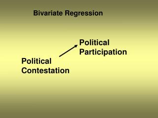
Bivariate Regression Analysis. The beginning of many types of regression. TOPICS. Beyond Correlation Forecasting Two points to estimate the slope Meeting the BLUE criterion The OLS method. Purpose of Regression Analysis. Test causal hypotheses Make predictions from samples of data

E N D
Bivariate Regression Analysis The beginning of many types of regression
TOPICS • Beyond Correlation • Forecasting • Two points to estimate the slope • Meeting the BLUE criterion • The OLS method
Purpose of Regression Analysis • Test causal hypotheses • Make predictions from samples of data • Derive a rate of change between variables • Allows for multivariate analysis
Goal of Regression • Draw a regression line through a sample of data to best fit. • This regression line provides a value of how much a given X variable on average affects changes in the Y variable. • The value of this relationship can be used for prediction and to test hypotheses and provides some support for causality.
Perfect relationship between Y and X: X causes all change in Y Where a = constant, alpha, or intercept (value of Y when X= 0 ; B= slope or beta, the value of X Imperfect relationship between Y and X E = stochastic term or error of estimation and captures everything else that affects change in Y not captured by X
The Intercept • The intercept estimate (constant) is where the regression line intercepts the Y axis, which is where the X axis will equal its minimal value. • In a multivariate equation (2+ X vars) the intercept is where all X variables equal zero.
The Intercept The intercept operates as a baseline for the estimation of the equation.
The Slope • The slope estimate equals the average change in Y associated with a unit change in X. • This slope will not be a perfect estimate unless Y is a perfect function of X. If it was perfect, we would always know the exact value of Y if we knew X.
The Least Squares Concept • We draw our regression lines so that the error of our estimates are minimized. When a given sample of data is normally distributed, we say the data are BLUE. • BLUE stands for Best Linear Unbiased Estimate. So, an important assumption of the Ordinary Least Squares model (basic regression) is that the relationship between X variables and Y are linear.
Do you have the BLUES? The BLUE criterion • B for Best (Minimum error) • L for Linear (The form of the relationship) • U for Un-bias (does the parameter truly reflect the effect?) • E for Estimator
The Least Squares Concept • Accuracy of estimation is gained by reducing prediction error, which occurs when values for an X variable do not fall directly on the regression line. • Prediction error = observed – predicted or
NOT BLUE BLUE
Ordinary Least Square (OLS) • OLS is the technique used to estimate a line that will minimize the error. The difference between the predicted and the actual values of Y
OLS • Equation for a population • Equation for a sample
The Least Squares Concept • The goal is to minimize the error in the prediction of b. This means summing the errors of each prediction, or more appropriately the Sum of the Squares of the Errors. SSE =
The Least Squares and b coefficient • The sum of the squares is “least” when • And Knowing the intercept and the slope, we can predict values of Y given X.
Step by step • Calculate the mean of Y and X • Calculate the errors of X and Y • Get the product (multiply) • Sum the products
Step by step • Squared the difference of X • Sum the squared difference • Divide (step4/step6) • Calculate a
Forecasting Home Values Y2 - Y1 _______ X2 - X1 4.54 – 3.53 __________ =.69 5.2 – 4.5
SPSS OUTPUT • The coefficient beta is the marginal impact of X on Y (derivative) • In other words for a one unit change of X how much Y changes (.575)
Stochastic Term • The stochastic error term measures the residual variance in Y not covered by X. • This is akin to saying there is measurement error and our predictions/models will not be perfect. • The more X variables we add to a model, the lower the error of estimation.
Interpreting a Regression • The prior table shows that with an increase in unemployment of one unit (probably measured as a percent), the S&P 500 stock market index goes down 69 points, and this is statistically significant. • Model Fit: 37.8% of variability of Stocks predicted by change in unemployment figures.
Interpreting a Regression 2 • What can we say about this relationship regarding the effect of X on Y? • How strongly is X related to Y? • How good is the model fit?
Model Fit: Coefficient of Determination • R squared is a measure of model fit. • What amount of variance in Y is explained by X variable? • What amount of variability in Y not explained by X variable(s)?
This measure is based on the degree to which the point estimates of fall on the regression line. The higher the error from the line, the lower the R square (scale between 1 and 0). = Total sum of squared deviations (TSS) = regression (explained) sum of squared deviations (RSS) = error (unexplained) sum of squared deviations (ESS) TSS= RSS + ESS Where R2 = RSS/TSS
Interpreting a Regression 2 • The correlation between X and Y is weak (.133). This is reflected in the bivariate correlation coefficient but also picked up in model fit of .018. What does this mean? • However, there appears to be a causal relationship where urban population increases democracy, and this is a highly significant statistical relationship (sig.= .000 at .05 level)
Interpreting a Regression 2 • Yet, the coefficient 4.176E-05 means that a unit increase in urban pop increases democracy by .00004176, which is tiny. • This model teaches us a lesson: We need to pay attention to both matters of both statistical significance but also matters of substance. In the broader picture urban population has a rather minimal effect on democracy.
The Inference Made • As with some of our earlier models, when we interpret the results regarding the relationship between X and Y, we are often making an inference based on a sample drawn from a population. The regression equation for the population uses different notation: Yi = α + βXi + εi
OLS Assumptions • No specification error • Linear relationship between X and Y • No relevant X variables excluded • No irrelevant X variables included • No Measurement Error • (self-evident I hope, otherwise what would we be modeling?)
OLS Assumptions • On Error Term: a. Zero mean: E(εi2), meaning we expect that for each observation the error equals zero. b. Homoskedasticity: The variance of the error term is constant for all values of Xi. c. No autocorrelation: The error terms are uncorrelated. d. The X variable is uncorrelated with the error term e. The error term is normally distributed.
OLS Assumptions • Some of these assumptions are complex and issues for a second level course (autocorrelation, heteroskedasticity). • Of importance is that when assumptions 1 and 3 are met our regression model is BLUE. The first assumption is related to the proper model specification. When aspects of assumption 3 are violated we may likely need a new method of estimation besides OLS