Download
1 / 39
420 likes | 807 Views
Bivariate linear regression. ASW, Chapter 12. Economics 224 – Notes for November 12, 2008 . Regression line. For a bivariate or simple regression with an independent variable x and a dependent variable y , the regression equation is y = β 0 + β 1 x + ε .

E N D
Bivariate linear regression ASW, Chapter 12 Economics 224 – Notes for November 12, 2008
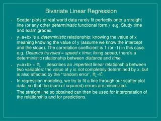
Regression line • For a bivariate or simple regression with an independent variable x and a dependent variable y, the regression equation is y = β0 + β1 x + ε. • The values of the error term, ε, average to 0 so E(ε) = 0 and E(y) = β0 + β1 x. • Using observed or sample data for values of x and y, estimates of the parameters β0 and β1 are obtained and the estimated regression line is where is the value of y that is predicted from the estimated regression line.
ε or error term Bivariate regression line y =β0 + β1x + ε y E(y) =β0 + β1x yi E(yi) x xi
y (actual) ŷ (estimated) deviation Observed scatter diagram and estimated least squares line y ŷ = b0 + b1x x
Example from SLID 2005 • According to human capital theory, increased education is associated with greater earnings. • Random sample of 22 Saskatchewan males aged 35-39 with positive wages and salaries in 2004, from the Survey of Labour and Income Dynamics, 2005. • Let x be total number of years of school completed (YRSCHL18) and y be wages and salaries in dollars (WGSAL42). Source: Statistics Canada, Survey of Labour and Income Dynamics, 2005 [Canada]: External Cross-sectional Economic Person File [machine readable data file]. From IDLS through UR Data Library.
YRSCHL18 is the variable “number of years of schooling” WGSAL42 is the variable “wages and salaries in dollars, 2004”
y y Mean of y is $45,954 and sd is $21,960. n = 22 cases Mean of x is 14.2 and sd is 2.64 years. x x
y x
Analysis and results H0: β1 = 0. Schooling has no effect on earnings. H1: β1 > 0. Schooling has a positive effect on earnings. From the least squares estimates, using the data for the 22 cases, the regression equation and associate statistics are: y = -13,493 + 4,181 x. R2 = 0.253, r = 0. 503. Standard error of the slope b0 is 1,606. t = 2.603 (20 df), significance = 0.017. At α = 0.05, reject H0, accept H1 and conclude that schooling has a positive effect on earnings. Each extra year of schooling adds $4,181 to annual wages and salaries for those in this sample. Expected wages and salaries for those with 20 years of schooling is -13,493 + (4,181 x 20) = $70,127.
Equation of a line • y = β0 + β1x. x is the independent variable (on horizontal) and y is the dependent variable (on vertical). • β0 and β1 are the two parameters that determine the equation of the line. • β0 is the y intercept – determines the height of the line. • β1 is the slope of the line. • Positive, negative, or zero. • Size of β1 provides an estimate of the manner that x is related to y.
Δy Δx Positive Slope: β1 > 0 y Example – schooling (x) and earnings (y). β0 x
Δx Δy Negative Slope: β1 < 0 y β0 Example – higher income (x) associated with fewer trips by bus (y). x
Δx Zero Slope: β1 = 0 y β0 Example – amount of rainfall (x) and student grades (y) x
Infinite number of possible lines can be drawn. Find the straight line that best fits the points in the scatter diagram.
Least squares method (ASW, 469) • Find estimates of β0 and β1 that produce a line that fits the points the best. • The most commonly used criterion is least squares. • The least squares line is the unique line for which the sum of the squares of the deviations of the y values from the line is as small as possible. • Minimize the sum of the squares of the errors ε. • Or, equivalent to this, minimize the sum of the squares of the differences of the y values from the values of E(y). That is, find b0 and b1 that minimize:
Least squares line • Let the n observed values of x and y be termed xi and yi, where i = 1, 2, 3, ... , n. • ∑ε2 is minimized when b0 and b1 take on the following values:
Is alcohol a superior good? Income is family income in thousands of dollars per capita, 1986. (independent variable) Alcohol is litres of alcohol consumed per person 15 years of age or over, 1985-86. (dependent variable)
Hypotheses H0: β1 = 0. Income has no effect on alcohol consumption. H1: β1 > 0. Income has a positive effect on alcohol consumption.
Analysis. b1 = 0.276 and its standard error is 0.076, for a t value of 3.648. At α = 0.01, the null hypothesis can be rejected (ie. with H0, the probability of a t this large or larger is 0.0065) and the alternative hypothesis accepted. At 0.01 significance, there is evidence that alcohol is a superior good, ie. that income has a positive effect on alcohol consumption.
Uses of regression line • Draw line – select two x values (eg. 26 and 36) and compute the predicted y values (8.1 and 10.8, respectively). Plot these points and draw line. • Interpolation. If a city had a mean income of $32,000, the expected level of alcohol consumption would be 9.7 litres per capita.
Extrapolation • Suppose a city had a mean income of $50,000 in 1986. From the equation, expected alcohol consumption would be 14.6 litres per capita. • Cautions: • Model was tested over the range of income values from 26 to 36 thousand dollars. While it appears to be close to a straight line over this range, there is no assurance that a linear relation exists outside this range. • Model does not fit all points – only 62% of the variation in alcohol consumption is explained by this linear model. • Confidence intervals for prediction become larger the further the independent variable x is from its mean.
Change in y resulting from change in x Estimate of change in y resulting from a change in x is b1. For the alcohol consumption example, b1 = 0.276. A 10.0 thousand dollar increase in income is associated with a 2.76 per litre increase in annual alcohol consumption per capita, at least over the range estimated. This can be used to calculate the income elasticity for alcohol consumption.
Goodness of fit (ASW, 12.3) • y is the dependent variable, or the variable to be explained. • How much of y is explained statistically from the regression model, in this case the line? • Total variation in y is termed the total sum of squares, or SST. • The common measure of goodness of fit of the line is the coefficient of determination, the proportion of the variation or SST that is “explained” by the line.
SST or total variation of y Value of y “explained” by the line Difference from mean “Error” of prediction Difference of any observed value of y from the mean is the difference between the observed and predicted value plus the difference of the predicted value from the mean of y. From this, it can be proved that: SST= Total variation of y SSE = “Unexplained” or “error” variation of y SSR = “Explained” variation of y
Variation in y y ŷ = b0 + b1x yi ŷi x xi
Variation in y “explained” by the line y ŷ = b0 + b1x yi ŷi “Explained” portion x xi
Variation in y that is “unexplained” or error ‘Unexplained” or error y yi – ŷi ŷ = b0 + b1x yi ŷi x xi
Coefficient of determination The coefficient of determination, r2or R2 (the notation used in many texts),is defined as the ratio of the “explained” or regression sum of squares, SSR, to the total variation or sum of squares, SST. The coefficient of determination is the square of the correlation coefficient r. As noted by ASW (483), the correlation coefficient, r, is the square root of the coefficient of determination, but with the same sign (positive or negative) as b1.
Interpretation of R2 • Proportion, or percentage if multiplied by 100, of the variation in the dependent variable that is statistically explained by the regression line. • 0 R2 1. • Large R2 means the line fits the observed points well and the line explains a lot of the variation in the dependent variable, at least in statistical terms. • Small R2 means the line does not fit the observed points very well and the line does not explain much of the variation in the dependent variable. • Random or error component dominates. • Missing variables. • Relationship between x and y may not be linear.
How large is a large R2? • Extent of relationship – weak relationship associated with low value and strong relationship associated with large value. • Type of data • Micro/survey data associated with small values of R2. For schooling/earnings example, R2 = 0.253. Much individual variation. • Grouped data associated with larger values of R2. In income/alcohol example, R2 = 0.625. Grouping averages out individual variation. • Time series data often results in very high R2. In consumption function example (next slide), R2 = 0.988. Trends often move together.
Consumption (y) and GDP (x), Canada, 1995 to 2004, quarterly data Consumption GDP
Beware of R2 • Difficult to compare across equations, especially with different types of data and forms of relationships. • More variables added to model can increase R2. Adjusted R2 can correct for this. ASW, Chapter 13. • Grouped or averaged observations can result in larger values of R2. • Need to test for statistical significance. • We want good estimates of β0andβ1, rather than high R2. • At the same time, for similar types of data and issues, a model with a larger value of R2 may be preferable to one with a smaller value.
Next day • Assumptions of regression model. • Testing for statistical significance.