Download

1 / 27
280 likes | 617 Views
Bivariate analysis. HGEN619 class 2007. Univariate ACE model. Expected Covariance Matrices. Bivariate Questions I. Univariate Analysis: What are the contributions of additive genetic, dominance/shared environmental and unique environmental factors to the variance?

E N D
Bivariate analysis HGEN619 class 2007
Bivariate Questions I • Univariate Analysis: What are the contributions of additive genetic, dominance/shared environmental and unique environmental factors to the variance? • Bivariate Analysis: What are the contributions of genetic and environmental factors to the covariance between two traits?
Bivariate Questions II • Two or more traits can be correlated because they share common genes or common environmental influences • e.g. Are the same genetic/environmental factors influencing the traits? • With twin data on multiple traits it is possible to partition the covariation into its genetic and environmental components • Goal: to understand what factors make sets of variables correlate or co-vary
Bivariate Twin Data (cross-twin within-trait) covariance (within-twin within-trait co)variance (cross-twin within-trait) covariance cross-twin cross-trait covariance
Bivariate Twin Covariance Matrix VX1 CX1X2 CX2X1 VX2 CX1Y1 CX2Y2 CX1Y2 CX2Y1 CY1X1 CY2X2 CY1X2 CY2X1 VY1 CY1Y2 CY2Y1 VY2
MZ Twin Covariance Matrix a112+e112 a112 a21*a11+ e21*e11 a222+a212+ e222+e212 a21*a11 a222+a212
DZ Twin Covariance Matrix a112+e112 .5a112 a21*a11+ e21*e11 a222+a212+ e222+e212 .5a21*a11 .5a222+ .5a212
Cross-Trait Covariances • Within-twin cross-trait covariances imply common etiological influences • Cross-twin cross-trait covariances imply familial common etiological influences • MZ/DZ ratio of cross-twin cross-trait covariances reflects whether common etiological influences are genetic or environmental
Practical Example I • Dataset: MCV-CVT Study • 1983-1993 • BMI, skinfolds (bic,tri,calf,sil,ssc) • Longitudinal: 11 years • N MZF: 107, DZF: 60
Practical Example II • Dataset: NL MRI Study • 1990’s • Working Memory, Gray & White Matter • N MZFY: 68, DZF: 21
! Bivariate ACE model! NL mri data I • #NGroups 4 • #define nvar 2 ! N dependent variables per twin • G1: Model Parameters • Calculation • Begin matrices; • X Lower nvar nvar Free ! additive genetic path coefficient • Y Lower nvar nvar Free ! common environmental path coefficient • Z Lower nvar nvar Free ! unique environmental path coefficient • H Full 1 1 ! • G Full 1 nvar Free ! means • End matrices; • Matrix H .5 • Start .5 X 1 1 1 Y 1 1 1 Z 1 1 1 • Start .7 X 1 2 2 Y 1 2 2 Z 1 2 2 • Matrix G 6 7 • Begin algebra; • A= X*X'; ! additive genetic variance • C= Y*Y'; ! common environmental variance • E= Z*Z'; ! unique environmental variance • V= A+C+E; ! total variance • S= A%V | C%V | E%V ; ! standardized variance components • End algebra; • Labels Row V WM BBGM • Labels Column V A1 A2 C1 C2 E1 E2 • End nlmribiv.mx
G2: MZ twins Data NInputvars=8 ! N inputvars per family Missing=-2.0000 ! missing values ='-2.0000' Rectangular File=mri.rec Labels fam zyg mem1 gm1 wm1 mem2 . . Select if zyg =1 ; Select gm1 wm1 gm2 wm2 ; Begin Matrices = Group 1; Means G| G; ! model for means, assuming mean t1=t2 Covariances ! model for MZ variance/covariances A+C+E | A+C _ A+C | A+C+E ; Options RSiduals End G3: DZ twins Data NInputvars=8 Missing=-2.0000 Rectangular File=mri.rec Labels fam zyg mem1 gm1 wm1 mem2 . . Select if zyg =2 ; Select gm1 wm1 gm2 wm2 ; Begin Matrices = Group 1; Means G| G; ! model for means, assuming mean t1=t2 Covariances ! model for DZ variance/covariances A+C+E | H@A+C _ H@A+C | A+C+E ; Options RSiduals End ! Bivariate ACE model! NL mri data II nlmribiv.mx
! Bivariate ACE model! NL mri data III • G4: summary of relevant statistics • Calculation • Begin Matrices = Group 1 • Begin Algebra ; • R= \stnd(A)| \stnd(C)| \stnd(E); ! calculates rg|rc|re • End Algebra ; • Interval @95 S 1 1 1 S 1 1 3 S 1 1 5 ! CI's on A,C,E for first phenotype • Interval @95 S 1 2 2 S 1 2 4 S 1 2 6 ! CI's on A,C,E for second phenotype • Interval @95 R 4 2 1 R 4 2 3 R 4 2 5 ! CI's on rg, rc, re • End nlmribiv.mx