Download
1 / 61
610 likes | 803 Views
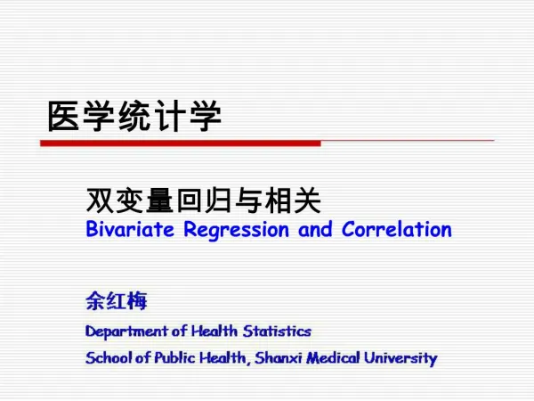
bivariate EDA and regression analysis. width. length. weight of core. distance from quarry. “scatterplot matrix”. scatterplots. scatterplots provide the most detailed summary of a bivariate relationship , but they are not concise , and there are limits to what else you can do with them…

E N D
width length
weight of core distance from quarry
scatterplots • scatterplots provide the most detailed summary of a bivariate relationship, but they are not concise, and there are limits to what else you can do with them… • simpler kinds of summaries may be useful • more compact; often capture less detail • may support more extended mathematical analyses • may reveal fundamental relationships…
y = a + bx 6 5 (x2,y2) 4 3 y (x1,y1) 2 x 1 1 2 3 4 5 6 b = “slope” b = y/xb = (y2-y1)/(x2-x1) a = “y intercept”
y = a + bx • we can predict values of y from values of x • predicted values of y are called “y-hat” • the predicted values (y) are often regarded as “dependent” on the (independent) x values • try to assign independent values to x-axis, dependent values to the y-axis…
y = a + bx • becomes a concise summary of a point distribution, and a model of a relationship • may have important explanatory and predictive value
how do we come up with these lines? • various options: • by eye • calculating a “Tukey Line” (resistant to outliers) • ‘locally weighted regression’ – “LOWESS” • least squares regression
linear regression • linear regression and correlation analysis are generally concerned with fitting lines to real data • least squares regression is one of the main tools • attempts to minimize deviation of observed points from the regression line • maximizes its potential for prediction
standard approach minimizes the squared variation in y • Note: • these are the vertical deviations • this is a “sum-squared-error approach”
regressing x on y would involve defining the line by minimizing
calculating a line that minimizes this value is called “regressing y on x” • appropriate when we are trying to predict y from x • this is also called “Model I Regression”
start by calculating the slope (b): covariance
once you have the slope, you can calculate the y-intercept (a):
regression “pathologies” • things to avoid in regression analysis
Tukey Line • resistant to outliers • divide cases into thirds, based on x-axis • identify the median x and y values in upper and lower thirds • slope (b)= (My3-My1)/(Mx3-Mx1) • intercept (a) = median of all values yi-b*xi
Correlation • regression concerns fitting a linear model to observed data • correlation concerns the degree of fit between observed data and the model... • if most points lie near the line: • the ‘fit’ of the model is ‘good’ • the two variables are ‘strongly’ correlated • values of y can be ‘well’ predicted from x
“Pearson’s r” • this is assessed using the product-moment correlation coefficient: = covariance (the numerator), standardized by a measure of variation in both x and y
+ + - - (xi,yi)
unlike the covariance, r is unit-less • ranges between –1 and 1 • 0 = no correlation • -1 and 1 = perfect negative and positive correlation (respectively) • r is symmetrical • correlation between x and y is the same as between y and x • no question of independence or dependence… • recall, this symmetry is not true of regression…
regression/correlation • one can assess the strength of a relationship by seeing how knowledge of one variable improves the ability to predict the other
if you ignore x, the best predictor of y will be the mean of all y values (y-bar) • if the y measurements are widely scattered, prediction errors will be greater than if they are close together • we can assess the dispersion of y values around their mean by:
r2= • “coefficient of determination” (r2) • describes the proportion of variation that is “explained” or accounted for by the regression line… • r2=.5 half of the variation is explained by the regression… half of the variation in y is explained by variation in x…
correlation and percentages • much of what we want to learn about association between variables can be learned from counts • ex: are high counts of bone needles associated with high counts of end scrapers? • sometimes, similar questions are posed of percent-standardized data • ex: are high proportions of decorated pottery associated with high proportions of copper bells?
caution… • these are different questions and have different implications for formal regression • percents will show at least some level of correlation even if the underlying counts do not… • ‘spurious’ correlation (negative) • “closed-sum” effect
10 vars. 5 vars. 3 vars. 2 vars.
original counts percents (10 vars.) percents (5 vars.) percents (3 vars.) percents (2 vars.)
regression assumptions • both variables are measured at the interval scale or above • variation is the same at all points along the regression line (variation is homoscedastic)
residuals • vertical deviations of points around the regression • for case i, residual = yi-y-hati [yi-(a+bxi)] • residuals in y should not show patterned variation either with x or y-hat • normally distributed around the regression line • residual error should not be autocorrelated (errors/residuals in y are independent…)
standard error of the regression • recall: ‘standard error’ of an estimate (SEE) is like a standard deviation • can calculate an SEE for residuals associated with a regression formula
to the degree that the regression assumptions hold, there is a 68% probability that true values of y lie within 1 SEE of y-hat • 95% within 2 SEE… • can plot lines showing the SEE… • y-hat = a+bx +/- SEE
data transformations and regression • read Shennan, Chapter 9 (esp. pp. 151-173)