Download
1 / 35
350 likes | 533 Views
Bivariate Regression. Assumptions and Testing of the Model. Economics 224, Notes for November 17, 2008. Assignments. Assignment 6 is optional. It will be handed out next week and due on December 5. If you are satisfied with your grades on Assignment 1-5, then you need not do Assignment 6.

E N D
Bivariate Regression Assumptions and Testing of the Model Economics 224, Notes for November 17, 2008
Assignments • Assignment 6 is optional. It will be handed out next week and due on December 5. • If you are satisfied with your grades on Assignment 1-5, then you need not do Assignment 6. • If you do Assignment 6, then we will base your mark for the assignments on the best five marks.
Corrections from last day • Significance of t values from Excel are for two-tailed or two-directional tests. • If alternative hypothesis is one-directional, that is, lesser than or greater than, then cut the P-value in half. • I used H1 as the name of the alternative hypothesis. The text uses Ha, so I will use that from now on.
Example: The Consumption Function • A key part of the Keynesian aggregate expenditure model. • Let C = aggregate consumption and Y = aggregate demand • Key role of the marginal propensity to consume (MPC) out of real GDP = ∆C/∆Y. • Estimating C = β0 + β1Y + ε. • Data set posted on UR Courses. • Find estimates b1 of the slope β1 and b0 of intercept β0 to produce an estimate of the consumption function: • In a revised model, you might use total income or disposable income for Y and include other relevant variables.
Hypotheses • H0: β1 = 0. Real GDP has no relation to consumption or MPC = 0. • Ha: β1 > 0. Real GDP has a positive relationship with consumption or MPC > 0.
Consumption Real GDP
Statistics from Excel for regression of consumption on real GDP
Analysis of consumption function results • The t test for the regression coefficient gives a t value of 55.1, with probability extremely small (7.03 times 10 to the power of minus 38). The null hypothesis of real GDP having no relationship with consumption is rejected and the alternative hypothesis that consumption has a positive relationship with real GDP is accepted. • The estimate of the slope, in this case the MPC, is 0.532. Over this period, increases in real GDP are associated with increases in consumption of just over one-half of GDP. • There appears to be serial correlation in the model (see later slides) so the assumptions are violated. This violation may not affect the estimate of the MPC all that much. • Time series regressions of this type often have a very good fit to the data. In this case, R2 = 0.988.
Assumptions for regression model • Linear relationship between x and y. • Transform curvlinear relation to a linear one. • Interval or ratio level scales for x and y. • Nominal scales – dummy variables and multiple regression. • Ordinal scales – be very cautious with interpretation. • x truly independent, exogenous, and error free. • May correct for latter with an errors in variables model. • No relevant variables excluded from the model. • Several assumptions about the error term ε. • Random variable with mean of 0. • Normally distributed random errors. • Equal variances. • Values of ε independent of each other.
Error term ε in • Importance • Source of information for statistical tests. • Violation of assumptions may mean regression model, estimates, and statistical tests inaccurate. • Source of error • Random component – random sampling, unpredictable individual behaviour. • Measurement error. • Variables not in equation. • Examination of residuals provides possibility of testing assumptions about ε (ASW, 12.8).
Assumptions about ε (ASW, 487-8) • E(ε) = 0. ε is a random error with a mean or expected value of zero so that E(y) = β0+ β1x is the “true” regression equation. • Var(ε) = σ2for each value of x. For different values of x, the variance for the distribution of random errors is the same. This characteristic is referred to as homoskedasticity and if this assumption is not met, the model has heteroskedasticity. • Values of ε are independent of each other. For any x, the values of ε are unrelated to or independent of values of ε for any other x. The violation of this assumption may be referred to as serial correlation or autocorrelation. • For each x, the distribution of values of ε is a normal distribution.
Assumptions in practice • These strong assumptions about the random error term ε are often not met. Econometricians have developed many procedures for handling data where assumptions are not met. • For testing the model, assume the assumptions are met. • If the assumptions are met, econometricians show that the least-squares estimators are the best linear unbiased estimators (BLUE) possible.
Assumptions in examples • Regression of wages and salaries on years of schooling. Microdata from a random sample means that the errors are likely random with mean 0 and are likely independent of each other. Distribution of wages and salaries may not be normal and variance of wages and salaries at different years of schooling may not be equal. • Consumption function likely has correlated errors associated with it and may not meet the equal variance and normal distribution assumptions. But estimate of MPC may be reasonably accurate. • Alcohol example probably violates each assumption somewhat. However, the estimate of the effect of income on alcohol consumption may be a reasonable estimate.
Testing the model for statistical significance • The key question is whether the slope is 0 or not, that is, whether the regression model explains any of the variation in the dependent variable y. The hypotheses are: H0: β1 = 0. Ha: β1 ≠ 0. • If the true relationship is y = β0 + β1x + ε, different samples yield different values for the estimators b0 and b1 of the parameters β0 and β1, respectively. With repeated sampling, these estimators thus have a variability or standard error. This variability depends on the variability of the random error term so estimating σ2 is the first step in testing the model. • There are two tests, the t-test for the statistical significance of the slope and the F-test for the significance of the equation. For bivariate regression, these two tests give identical results, but they are different tests in multivariate regression.
Estimating σ2, the variance of ε • The values of the random error term ε are not observed but, once a regression line has been estimated from a sample, the residuals (ei) can be calculated and used to construct an estimate of σ2. Recall that the error sum of squares, or unexplained variation, was SSE. • Dividing SSE by the degrees of freedom provides an estimate of the variance. This is termed the mean square error (MSE) and, for a bivariate regression line, equals • There are n – 2 degrees of freedom since two parameters, β0 and β1, are estimated in a bivariate regression.
Standard error of estimate s or se • Associated with each regression line is a standard error of estimate. ASW use the symbol s. Some texts use the symbol se to distinguish it from the standard deviation of a variable. • Alcohol example. N=10, SSE = 4.159933, MSE = SSE/8 = 0.519992. and note this is given in Excel Regression Statistics box. • Schooling and earnings. s = 19,448. See next slides.
Standard error of estimate s or se • Rough rule of thumb: • Two-thirds of observed values are within 1 standard error of estimate of the line. • 95% plus of observed values are within 2 standard errors of the line. Standard error of estimate Two standard errors of estimate
2 st. errors 1 st. error y 15 /22 observations within 1 st. error and 21/22 within 2 st. errors
Distribution of b1 • The statistic b1 has a mean of β1, ie. E(b1) = β1. • Standard error of b1 is the standard error or estimate divided by the square root of the variation of x. The estimate of this standard error is • The distribution of b1 is described by a t-distribution with the above mean and standard deviation and n-2 degrees of freedom.
Schooling and earnings example – standard error of the slope.
Test of statistical significance for b1 H0: β1 = 0. Ha: β1 ≠ 0. • b1 is the test statistic for the hypotheses and the t value, with n-2 df, is Since the null hypothesis is usually that β1 = 0, this becomes b1 divided by its standard deviation or standard error. • Schooling and earnings example. and, with a sample of n = 22 cases, there are 22 - 2 = 20 df. The result is statistically significant at the α = 0.02 level of significant (P-value = 0.017). Reject H0 and accept Ha. Schooling associated with earnings at 0.02 significance.
If test t-value outside the range → reject H0. Reject H0 Reject H0 Do Not Reject H0 a/2 = .025 a/2 = .025 z 0 t0.025 ≈ 2.0 t0.025 ≈ 2.0
Rule of thumb of 2 • Since the null hypothesis is usually H0: β1 = 0, • The question is how large a t value is necessary to reject this hypothesis. • When the degrees of freedom is large, the t distribution approaches the normal distribution. At α = 0.05, for a two-tailed test, the critical values are t or Z of -1.96 and +1.96. • Thus, for large samples or for data sets with many observations (say 100 plus), if b1 is over double the value of sb1, reject H0 and accept Ha. If b1 is less than twice the value of sb1, do not reject H0. • This is just a rough rule of thumb. • Where df < 50, it is best to check the P-value associated with the t value.
Test for the intercept • A parallel test can be conducted for the intercept of the line. Given that economic theory often is silent on the issue of what the intercept might be, this is usually of little interest. • If there is reason to hypothesize a value for the intercept, follow the same procedure. The Excel estimate of the regression coefficients provides the estimator of the slope, its standard error, t-value, and P-value.
Confidence interval for b1 • From the distribution for b1, interval estimates for estimates of β1 are formed as follows: • For the schooling and earnings example, b1 = 4,181, the standard error of b1 = 1,606, and n = 22, so t for 20 df and 95% confidence is tα/2 = t0.05 = 2.086, giving the interval from 831 to 7,531 – a wide interval for estimate of the effect of an extra year of schooling on annual wages and salaries.
F test for R2 H0: β1 = 0 or R2 = 0. No relationship. Ha: β1 ≠ 0 or R2 ≠ 0. Relationship exists. • Test is the ratio of the regression mean square to the error mean square, an F test. • Reject H0 and accept Ha if F is large, ie. P-value associated with F is below the value of α selected (eg. 0.05). • Do not reject H0 if F is not large, ie. P-value associated with F is above the level of α selected (eg. 0.05). • For a bivariate regression, this test is exactly equivalent to the t test for the slope of the line. • In multivariate regression, the F test provides a test for the existence of a relationship. The t test for each independent variable is a test for the possible influence of that variable.
Example – income and alcohol consumption H0: β1 = 0 or R2 = 0. No relationship between income and alcohol consumption. Ha: β1 ≠ 0 or R2 ≠ 0. Income affects alcohol consumption. • F = MSR/MSE = 6.920067 / 0.519992 = 13.308. P = 0.006513. Reject H0 and accept Ha at α = 0.01. • F table. At α = 0.01, with 1 and 8 df, F = 11.26. Estimated F = 13.30803 > 11.26. Reject H0 and accept Ha at 0.01 level. • At 0.01 significance, conclude that income affects alcohol consumption.
Example – schooling and earnings H0: R2 = 0. No relationship between years of schooling and wages and salaries. Ha: R2 ≠ 0. Years of schooling related to wages and salaries. R2 = 0.253 and the F value is 6.776 with 1 and 20 df. At α = 0.05, F = 4.35 for 1 and 20 df. Reject H0 and accept H1 at α = 0.05. P value = 0.017 so reject H0 at 0.02 significance but not at 0.01.
Estimation and prediction (ASW, 498-502) • Point estimate provided by estimated regression line. • In the example of the effect of years of schooling on wages and salaries, predicted wages and salaries for those with 16 years of schooling are: • The confidence intervals associated with the predicted values: • Depend on the confidence level (eg. 95%), the standard error, the sample size, the variation of x, and the distance x is from its mean. Formulae in ASW, pp. 499 and 501. • Greater distance of x from the mean of xassociated with a wider interval.
FIGURE 12.8 CONFIDENCE INTERVALS FOR THE MEAN SALES y AT GIVEN VALUES OF STUDENT POPULATION x
FIGURE 12.9 CONFIDENCE AND PREDICTION INTERVALS FOR SALES y AT GIVEN VALUES OF STUDENT POPULATION x
Example – Schooling and wages and salaries. Inner band gives 95% confidence intervals for prediction of mean values of wages and salaries for each year of schooling. Outer band gives 95% prediction intervals for individual wages and salaries. Se = 19,447 Sb1 = 1,606 t = 2.603 for slope and P-value = 0.017
Confidence intervals for estimation and prediction • For estimation of predicted mean value of the dependent variable, the inner bands illustrate the intervals. • For estimation of predicted individual values of the dependent variable, the outer bands illustrate the intervals. These intervals can be very large. In the above example they are so large that predicting individual wages and salaries from years of schooling is almost completely unreliable. But it is unrealistic to expect that a sample of size 22, with only one independent variable (years of schooling) would allow a good prediction of individual salaries. • Interval estimates can be narrowed by expanding sample size and constructing a model with improved fit and reduced standard error.
Wednesday • Reporting regression results. • Examination of residuals, ASW, 12.8. • Examples of transformations. • Introduction to multiple regression.