Download
1 / 15
150 likes | 349 Views
Single Cycle MIPS Implementation. All instructions take the same amount of time Signals propagate along longest path CPI = 1 Lots of operations happening in parallel Increment PC ALU Branch target computation Inefficient. Multicycle MIPS Implementation.

E N D
Single Cycle MIPS Implementation • All instructions take the same amount of time • Signals propagate along longest path • CPI = 1 • Lots of operations happening in parallel • Increment PC • ALU • Branch target computation • Inefficient
Multicycle MIPS Implementation • Instructions take different number of cycles • Cycles are identical in length • Share resources across cycles • E.g. one ALU for everything • Minimize hardware • Cycles are independent across instructions • R-type and memory-reference instructions do different things in their 4th cycles • CPI is 3,4, or 5 depending on instruction
Multicycle versions of various instructions • R-type (add, sub, etc.) – 4 cycles • Read instruction • Decode/read registers • ALU operation • ALU Result stored back to destination register. • Branch – 3 cycles • Read instruction • Get branch address (ALU); read regs for comparing. • ALU compares registers; if branch taken, update PC
Multicycle versions of various instructions • Load – 5 cycles • Read instruction • Decode/read registers • ALU adds immediate to register to form address • Address passed to memory; data is read into MDR • Data in MDR is stored into destination register • Store – 4 cycles • Read instruction • Decode/read registers • ALU adds immediate to a register to form address • Save data from the other source register into memory at address from cycle 3
Control for new instructions • Suppose we introduce lw2r: • lw2r $1, $2, $3: • compute address as $2+$3 • put result into $1. • In other words: lw $1, 0($2+$3) • R-type instruction • How does the state diagram change?
Control for new instructions • Suppose we introduce lw2r: • lw2r $1, $2, $3: • compute address as $2+$3 • Load value at this address into $1 • In other words: lw $1, 0($2+$3) • R-type instruction • How does the state diagram change? • New states: A,B,C • State 1 (op=‘lw2r’) State A State B State C back to 0 • A controls: ALUOp=00, ALUSrcA=1, ALUSrcB=0 • B controls: MemRead=1, IorD = 1 • C controls: RegDst = 1, RegWrite = 1, MemToReg = 1
Performance • CPI: cycles per instruction • Average CPI based on instruction mixes • Execution time = IC * CPI * C • Where IC = instruction count; C = clock cycle time • Performance: inverse of execution time • MIPS = million instructions per second • Higher is better • Amdahl’s Law:
Performance Examples • Finding average CPI:
Performance Examples • Finding average CPI: • CPI = 0.50*2 + 0.08*2 + 0.08*3 + 0.34*1 CPI = 1.74
Performance Examples • CPI = 1.74 • Assume a 2GHz P4, with program consisting of 1,000,000,000 instructions. • Find execution time
Performance Examples • CPI = 1.74, 2GHz P4, 10^9 instructions. • Execution_time = IC * CPI * Cycletime = 10^9 * 1.74 * 0.5 ns = 0.87 seconds
Performance Examples • We improve the design and change CPI of load/store to 1. • Speedup assuming the same program?
Performance Examples • We improve the design and change CPI of load/store to 1. • Speedup assuming the same program/cycle time? • CPInew = 0.5*1 + 0.08*2 + 0.08*3 + 0.34*1 CPInew = 1.24 • Speedup = 1.74/1.24 = 1.4
Amdahl’s Law • Suppose I make my add instructions twice as fast. • Suppose 20% of my program is doing adds • Speedup? • What if I make the adds infinitely fast?
Amdahl’s Law • Suppose I make my add instructions twice as fast. • Suppose 20% of my program is doing adds • Speedup? New Exectime = old_exectime(4/5 + (1/5)/2) = 9/10 * old_exectime Speedup = 10/9 • What if I make the adds infinitely fast? Speedup = 5/4, only 20% improvement!