Download
1 / 46
470 likes | 630 Views
The GBT Precision Telescope Control System. Kim Constantikes. Overview. The Green Bank Telescope Scientific Requirements and Objectives The Real Telescope Instrumentation Next Steps. Telescope Structure and Optics. Telescope Structure and Optics. Offset-Gregorian design

E N D
The GBT Precision Telescope Control System Kim Constantikes
Overview • The Green Bank Telescope • Scientific Requirements and Objectives • The Real Telescope • Instrumentation • Next Steps
Telescope Structure and Optics • Offset-Gregorian design • Operation to 115 GHz, 40 GHz winter 2003-2004 • Optics: 110 m x 100 m of a 208 m parent paraboloid • Effective diameter: 100 m • Off axis feedarm • F/D ~ 0.6 • Elevation Limit: 5° • Slew Rates: Azimuth - 40°/min; Elevation - 20°/min • Main Reflector: 2004 actuated panels with 68 m rms. • Total surface: rms 400 m • FWHM Beamwidth: 740"/f(Ghz) • Prime Focus: Retractable boom • Gregorian Focus: • 8-m elliptic subreflector with 6-degrees of freedom • Rotating Turret with 8 receiver bays • Typical 20-60 K Tsys, maximum efficiency 70-75%, NEDT 1 mK to 1 mK
Scientific Requirements • Efficiency/Collimation: Aperture error ~<1/16l • Maximize flux collected from unresolved source • Minimize background confusion, e.g., bright source in sidelobe • Best spatial sampling for mapping, e.g., think of beam shape as spatial impulse response • Pointing • Minimize calibration uncertainty of unresolved source intensity • Maximize collected flux • Accurate enough to find calibrator (blind) • Offset good enough over ~5° to find program source • Track stable over one-half hour
Pointing Coefficients Feed arm tip moves ~ 400mm as elevation changes from horizon to zenith: ~ 300 arcsec of elevation pointing ~ 100 mm of focus shift > 2 orders of magnitude improvement needed! Entire pointing error budget is: 0.32 mm subreflector X translation, or 0.41 mm subreflector Y translation, etc.
Approach • 2003 • Develop and test methods for astronomical characterizations of structure- pointing and efficiency- and collect data • Improvements in gravity model • Develop instruments and algorithms for thermal corrections, test and refine • Develop algorithms and test existing laser rangefinder system • 2004 • Implement additional instrumentation • Develop additional algorithms, test • Emphasize slow perturbations: Available servo bandwidth < 1 Hz (subreflector), dominant effects are ~ 0.1 Hz or less. • Have new pointing and surface corrections in place for winter 2004-2005: Objective of “good” 52 GHz, “Usable” 86 GHz
Pointing Degradation Mechanisms: Most are slow, < 0.1 Hz • Gravitational distortions, alignment: • Structure is linear (stress tensor), powerful constraint! • Compensate with “Traditional” pointing model: sin/cos of az,el (2-D Fourier series in general, “Condon Series”) • Thermal distortions (mostly gradient): • Mechanical design is “homologous”. Diurnal focus variation ~ 40 mm, elevation variation ~ 30 arcsec, worst transient around sunup, large effects persist to hours after sundown • Wind load distortions: • Predicted and measured pointing effects up to 10’s of arcsec • Structural vibrations (particularly at “jerky” scan start) • 10’s of arcsec • Azimuth track bumps, elevation anomaly ~ 5 arcsec • Servo errors, response to perturbations (wind, bumps) ~ 1-2 arcsec • Miscellaneous at <= 1 arcsec: Bearing wobble, encoder error… • Anomalous refraction at high frequencies
Efficiency Loss Mechanisms, Polarization Errors • Efficiency: • Uncompensated gravitational distortions, I.e., structural finite element model prediction errors • Uncompensated thermal distortions of back-up structure (also causes focus error) • Primary panel shape errors • Secondary figure errors • Mis-collimation • Polarization • Squint and Squash • Coupling
Surface errors ~300-400um rms; dominated by large scale errors. Traditional and “oof” measurements; consistent but complimentary results. Efficiency improvements of ~30-50% by quick, easy large-scale adjustments. Holography Results 150 x 150 pixel 12GHz traditional map 43GHz (SiO maser) OOF map
Successfully passed two design reviews Delivered Q Band (43GHz) performance: Blind pointing < 4” radial rms Offset pointing < 2.7” radial rms Focus < 2.5 mm rms 43% peak efficiency PTCS Technical Achievements Dynamic pointing corrections 43GHz gain-elevation curve Half-hour ½ power track, σ2 ~1”
Correcting Focus for Thermal Distortions • Corrected via robust linear regression of linearized features: • Temperature differences • Gravity model • Wind velocities in alidade-relative frame • Include k-nearest neighbor estimates of az, el anomalies • Current best model has 68% at < 2mm
The Real vs. Ideal GBT: Servo Effects and Structure Vibration
Predicting Tracking Error From Inclinometers Samples (10 Hz)
Instrumentation Structure Temperature Quadrant Detector Laser Structure Temperature Air Temperature IR Camera Structure Temperatures (4) 3-Axis Accelerometer Structure Temperatures (3) Air Temperature Structure Temperatures (2) Structure Temperatures (4) Air Temperature Structure Temperatures (2) Air Temperature Quadrant Detector 2-Axis Inclinometers (2) 3-Axis Accelerometers (2) Elevation Encoder Structure Temperatures (2) Structure Temperatures (2) Structure Temperatures (2) Air Temperature Azimuth Encoder
Inclinometers • 2-axis (horizontal plane), both elevation bearings • 0.1” short-term accuracy, 0.01” resolution • ~1 sec damping, 17 Hz resonance • 10 Hz sampling rate • Azimuth track maps • Real time measure/correct Az/El • Verify thermal effects • Wind force spring balance • Structural resonances
Accelerometers • 3-axis, elevation bearings and receiver cabin • MEMS torsion, capacitive readout, nickel • 2 micro-G/root Hz • 10 Hz sampling • 1 x 1 x 0.1 G dynamic range • 24 x 24 x 16 bit mixed signal ADC/microprocessor • Structural resonances • Receiver microphonics • Rate-aid inclinometers
Laser Rangefinders • 780 nm laser, 0.5 milliradian beam • 1.5 GHz CW modulation • Goal 100 micron accuracy • Variable integration time • Steerable beam, ~0.3 milliradian resolution • Position by trilateration • Primary figure adjustments • Collimation • Structural model data
Structural/Air Temperature Sensors • 0.15 C accuracy, -35 to 40 C • 0.05 C interchangable thermistors • 0.01 C resolution, 1 sec sampling • 19 structure sensors (soon 23) • 5 air sensors (forced convection cells, ~ 5 sec time constant) • Structure thermal distortions • Vertical air lapse • Laser rangefinder group index calculations
Quadrant Detector • 1 arcsec angle-angle measurements • ~5 Hz bandwidth, sampling at 10 Hz • Measurement noise ~ 0.2 arcsec (in lab) • Good relative measurements on ½ hour time scales • Degraded by turbulence, index gradients • Feed arm position/motion WRT ~elevation shaft (tipping structure coordinates) • Structural resonances
Infrared Thermography • 160 x 120 8-12 micron uncooled microbolometer array (Inframetrics) • 0.1 C resolution, accuracy = ? • Image primary mirror from feedarm • Primary surface coating black in long wave, Lambertian • Supporting temperature sensors on two panels, two adjacent locations in back-up structure (BUS) • Thermal gradients of mirror • Inferences of BUS gradients • Combine with OOF maps to refine FEM stiffness estimates of BUS • Regressions with OOF to get thermal distortions
Weather Stations, Servo Monitor • Three weather stations • Air temp, wind speed/direction, humidity, barometric pressure • Two on periphery of compound, one on feed arm tip • All drives are monitored • Currents and tachometers
Current Best Efficiency • Zernike corrections of primary using OOF maps: Improved 40° elevation efficiency (Q-band) by ~25 to 40% • Beam width reduced • Sidelobes attenuated
Current Best Pointing Models • Training on all data but test sets • Test sets: One “Track”, one all-sky run • Train results: 68th percentile residuals, all elevations, all winds, all hours-Focus: 2.2 mm, Elevation: 2.6”, Azimuth 3.6” • Track results: 68th percentile residuals, elevation 20-85, winds < 3.5 m/s, 0000-0800 EDT-Focus: 0.7 mmElevation: 1.9” (6” offset)Azimuth 2.8” (7” offset) • All-sky results: 68th percentile residuals, elevation 20-85, winds < 3.5 m/s, 0000-0800 EDT-Focus: 1.1 mmElevation: 2.3” (2” offset)Azimuth 2.6” (3” offset)
Technical Challenges 2004-2005 • Laser Rangefinders • Risk mitigation for other techniques • Improved rangefinder pointing • Improved ground and feedarm geometries: Larger acceptance angle retros (n=2 glass), cantilevered supports on feedarm • Next measurement campaign summer ’05 • Utilization of new instruments • System ID for inclinometers: Separate vibrations, azimuth drive hunting- attempt real time corrections for azimuth track and wind forces. Possibly directly to half-power track data… • IR Thermometry and OOF maps: Combined thermal/gravity enhancements of active surface control • Better characterization of pointing performance • Quantitative offset and track analysis: What are metrics? Can metrics be used for more sophisticated optimizations? Use for Monte-Carlo detection experiment design?
Technical Challenges 2004-2005 • Implement and test new pointing models, including • Wind effects • Azimuth track effects • Elevation anomaly • Start design of dense temperature sensor infrastructure- Increase sensors by x10? • Algorithms for improved trajectory shaping/control • Minimization of structure transients • Maximize observing time • Engineering tests of bolometer array may be possible in early spring 2005 • Great potential for investigating beam shape, optimizing efficiency, speed up OOF mapping. • Collect/analyze additional astronomical data on pointing, wavefront errors
Technical Challenges 2004-2005 • Thermal-mechanical FEM of BUS • Characterize main drive controls, investigate new control algorithms- Does modern control approach have advantages?
PTCS Project Team • Richard Prestage: Project Manager, Green Bank Site Deputy Director- Holography, Astronomy • Jim Condon: Project Scientist- Astronomy, Experimental Design/Analysis • Kim Constantikes: Project Engineer- Instrumentation, Algorithms, System Design, Pointing, etc. • ~ 9 Full time participants- 2 software engineers, 2 electrical engineers/technicians, 1 metrologist, 1 mechanical designer • Plus machine shop, mechanic, etc. support
Technical Activities Detailed characterization of offset pointing performance. Develop detailed error budgets: Attack in cost/benefit order. Corrections for wind pointing errors. Corrections for azimuth track uneveness. Develop instruments/ techniques for combined thermal/ gravity model of primary. Winter 04/05 goals Usable 86 GHz telescope: 1.7” offset pointing 0.28 mm surface error at night, wind < 2.5 m/s (50%) Good 52 GHz telescope: 2” offset pointing 0.35mm surface error extended environment (more sun, wind) PTCS Technical Challenges • Laser rangefinder improvements: • Pointing and geometry • Risk mitigation for alternatives
Approaches • Laser Metrology • Measure position of all relevant components to ~ 100 microns, infer orientations • Currently low-level and long time-line • Combined Astronomical, Structural Measurements, Models • Semi-empirical models driven by indirect measurements • E.g, astronomical pointing, linear regressions against suitable parameters: Temperature gradients, wind pressure, etc. • E.g., holography and linear structure model (very important!) to refine finite element structure model prediction of primary shape vs. elevation angle. • Incremental improvements, small capital investment
Main Drives • Azimuth: 1 drive/wheel, 4 wheels per truck, 4 trucks • Elevation: 8 drives (bull gear/pinion) • 0.3” per bit, azimuth and elevation encoders • Analog velocity (tach) and torque (current) loops • Digital position loop 50Hz sampling (10 Hz parabolic demand) • ~0.3 Hz closed loop bandwidth (< ~0.6 Hz first structural mode !) • Current loop lag-compensated, velocity loop lead-lag compensated, position loop type-II with nonlinear compensation for large angle motions • < 1” spec tracking error for constant velocity • Max 20 Deg/min elevation, 40 Deg/min azimuth
Subreflector Drive/Stage, Active Surface Control • Subreflector/six link “Stewart Platform” • Full 6DOF control • Magnetostrictive link length encoders • Spec xx translation accuracy, yy tilt accuracy • Active surface • 2209 actuators, DC motor drives, LVDTs • ~ 25 micron closed loop, ~ 75 micron accuracy (LVDT) • Cube retroreflector at near each panel corner
Example: Multilateration with laser rangefinders Graph state defined by edge data, Matlab engine retains state in global structures Can probe or break on edges, pause execution, and use full MATLAB IDE in paused state Hierarchical graphs modularize operators Graph edges carry primitive data types, structures, generic objects Graph nodes execute when input data are available Node parameters can be changed on the fly, parameters can be promoted to inputs, etc. Database operations via ODBC and SQL