Download
1 / 30
390 likes | 971 Views
Absorbing Boundary Conditions ( ABCs) (2 Sessions ) (1 Task). Absorbing Boundary Conditions (ABC). First-order ABCs are those which estimate value of fields outside boundary by looking back one step in time and one grid cell in space.

E N D
Absorbing Boundary Conditions (ABC) • First-order ABCs are those which estimate value of fields outside boundary by looking back one step in timeand one grid cell in space. • Higher order ABCs may look back over more steps in time and more grid cells in space. • In general, different ABCs are better suited for different applications. • Choice of particular ABC is also made by considering its numerical efficiency and stability. • Among different types of ABC, two particular: • Those based on one-way wave equations. • Those based on surrounding FDTD domain with a layer of absorbing material, essentially creating a numerical anechoic chamber. • Microwave dark rooms, or anechoic chambers, are constructed with walls completely covered with absorbing materials, often in corrugated form (for tapered impedance matching), designed to minimize reflections and thus make rooms suitable for testing antennas and other radiating devices. • One absorbing material is a lossy mixture of high-permeability ferrite material and a high-permittivity barium titanate material (ferrite-titanate), for which are complex as: • But magnitude of ratio. • Other is Perfectly Matched Layers (PML), will be considered.
Absorbing Boundary Conditions (ABC) • An example:
Absorbing Boundary Conditions (ABC) • Difference between a PECwall and a ABCwall: • ABC assumes that a PWS is incident on boundary. • and then estimates fields just outside boundary by using fields just inside the boundary. • However, this cannot be done withouterror since: • in most cases wave arriving at boundary is not exactly a PWS and is not normally incident. • ABCs are thus in general approximations, and reflect some of waves backintoFDTD space.
Absorbing Boundary Conditions (ABC) • ABCs based on one-way wave equation: • It depend on fact that solution of Maxwell’s coupled equations via an FDTD algorithm is equivalent to solution of second-order wave equation. • Although wave equation naturally supports propagating in both directions, it can be factored into two one-way wave equations. • This property provides basis for an algorithmic method by which fields can be “propagated out” of FDTD domain, minimizing reflections back into numerical space. • A first-order scheme of this type using 1D wave equation is known as first-order Mur boundary condition. • It is quite effective to remove onlynormally PWS on an FDTD boundary of 1D problems. • First-order Mur boundary: • It is simplest & effectiveABC for 1D simulations on normal incidence. • Mur ABC is based on one-way wave equations, or convection equations (CH3) as: • Hence the term “Radiation Boundary Conditions (RBC)” is used some time.
Absorbing Boundary Conditions (ABC) • ABC algorithms can be derived from one of them by using FDMdiscretization. • To derive ABC algorithms for left boundary, in terms of Ez and discretize it at x=Δx/2 (i.e., at mesh point i=3/2, just inside the boundary) and at time t=(n+1/2)Δt (i.e., at time index n+1/2): • Note that in FDTD algorithm, integerpoints are used and not available at half point i=3/2 & n+1/2. • Therefore a simple spatial averageis used as: • At rightmost edge of our 1D simulation space, with i=imax: average is i=3/2=1.5
Absorbing Boundary Conditions (ABC) • Second-order Mur: • First-order Mur works very well for 1D problems, where waves propagating is normalto boundary. • In 2D & 3D, waves are incident on boundaries at arbitrary angles and first-order Mur has lessaccurate. • For 2D wave equation: • Choice of wave equation depends on space &whichfieldcomponents are defined at boundary. • In other words, an ABC is only required for those field components for which normal update equations will not work, due to points falling outside boundary. • Consider 2D-TEcase, as illustrated in: • Along y=0boundary (i.e., j=1) we find only Exfield component, so a boundary condition based on a wave equation for Ex will be required; • But on x=0boundary, we find an Eyfield component, so a boundary condition based on a wave equation forEywill be required. • Alternatively, we could define boundary at Hz.
Absorbing Boundary Conditions (ABC) 1D wave Equation operators • Consider 2D-TMcase where Ezfalls on all boundaries: • We will need to consider waves incident on four walls of numerical space, as well as corners. • First, consider waves incident on left andright,i.e., at i=1 & imax, walls as illustrated in: • We can factor waves as follows: • For example, on rightmostedge of 2D grid: • Implementation at rightmost wall for 2D case is:
Absorbing Boundary Conditions (ABC) • Second-order Mur boundary condition in 2D at leftedge is: • Similar updateequations can be derived for other boundaries of 2D space, or can be simply transposed from above equation by modifyingsubscripts. • Second-orderMur boundary condition in 2D at bottomedge(j=1) is: • Disadvantage of second-order is that in addition to using field at time step n, prior values at time step (n−1)are required, and thus must be stored in memoryduringsimulation.
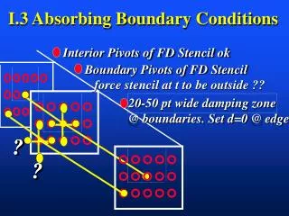
Absorbing Boundary Conditions (ABC) • Grid points used in Mur first & second-order boundaries are shown in: • In first-orderMur, apart from boundary point itself at previous time step, only point adjacent to boundary is used; as such it is no surprise that this boundary condition is only effective at normal incidence. • In second-order Mur boundary, all five surrounding points are used to update the boundary point
Absorbing Boundary Conditions (ABC) • Higher-order Mur boundaries: • First and second-order Mur boundaries leave reflections as shown in: • To reduce reflection, higher-order terms of Taylor series expansion is required. • Each of boundaries absorbs perfectly at normal incidence and reflects perfectly at grazing. • The performance improves with increasing order. • Instead, a method derived by Trefethen and Halpern [3] provides increased accuracy to Mur boundary without resorting to Taylor series expansion.
Absorbing Boundary Conditions (ABC) • Mur boundaries in 3D: • For Ezcomponent at x=0, we start from wave equation in 3D: • Similar to 2D, we can factor operator into and as: • Other radiation operators as ABCs: • Mur condition is just one of a number of examples of using radiation operators as absorbing boundaries. • & are radiation operators, which are applied in this case to electric field Ezat boundary. • In general, the idea in using radiation operators is to construct a PDE from a weighted sum of three types of derivatives of field components: • 1. Spatial derivatives in direction outward from FDTD space (∂/∂x in Mur derivation). • 2. Spatial derivatives in direction transverse to outward direction (∂/∂y). • 3. Temporal derivatives (∂/∂t). • Apart from Mur ABCs, a number of other radiation operator ABCs have been developed in short history of FDTD method. Where:
Absorbing Boundary Conditions (ABC) • Other Radiation Operators: • Bayliss-Turkel operators [6]: • It is based on time domain expressions for radiation far-field solutions of wave equation. • However, rather than using exact equations, they are presented in seriesexpansion form, for both spherical and cylindrical coordinates. • 2D cylindrical wave equation, for example for wave component Ezfor a 2D-TM mode, is given as: • Note that in cylindrical coordinates, unlike in Cartesian, we must define which coordinate is independent? • Wave propagate in rdirection for a cylindrical system can be expanded in a convergentseriesas: • Note that Bayliss-Turkeloperators are effective in cylindrical or spherical coordinates. no variations in z
Absorbing Boundary Conditions (ABC) • A. Sommerfeld, Partial Differential Equations in Physics, Academic Press, New York, New York, 1949. • Bayliss-Turkel Operators (cont.): • By using this, we can create a boundary that is far enough from origin so that higher-order terms become small compared to our desired error. • We now form differential operator as: • It is similar Mur boundary condition. • By applying this operator to previous equation, considering just first two terms of series: • Approximate one-way wave equation: • Which can be rewritten in: is known as the Sommerfeld radiation condition [7] can be neglected
Absorbing Boundary Conditions (ABC) • Bayliss-Turkel Operators (cont.): • This method would in general only work if fields are propagating exactlyin radialdirection, meaning they are normally incident on FDTD boundary. • Alternatively, if fields are not normal, one would have to use extensivecomputational and memory resources to make outer boundary very far from origin (which is presumably location of object of study, e.g., scatterer), so that neglecting higher order terms can be justified. • This limitation of normal incidence or very large computational space can be overcome with a slight modification to Sommerfeld radiation condition operator. (refer to related literatures). • Importance of Bayliss-Turkel type of radiation operators is that they are constructed without any knowledge of angular dependence of partial wave functions. • Spherical Coordinates: • Bayliss-Turkel operators can be constructed in spherical coordinates, using analogous methods [4, 8]. • Field component, for example Eφ, is expanded in following form:
Absorbing Boundary Conditions (ABC) • Previousconditions are effective at absorbing waves in specificscenarios, such as: • Murboundaries are effective at near normal incidence, • Bayliss-Turkeloperators are effective in cylindrical or spherical coordinates. • Aim is introduction a method to optimize absorption at a specific choice of incidentangles. • New method is based on R. L. Higdon’s idea, relies on a series of linear PDE for cancellation [9]. • Consider 2D plane waves having toward boundary in a 2D Cartesian FDTD space. • Assuming that components are propagating at angles from x-axis: • Superposition of such a wave structure is: • Numerical operator proposed by Higdonis: • Its particular advantage is that any combination of PWS toward x=0 wall at chosen discrete angles θmare completely absorbed. • For an incidence angle of θ=θm, Г is given by [9]: where: , and f(·) & g(·) are arbitrary functions for boundary at x=0
Absorbing Boundary Conditions (ABC) • Reflection coefficients for R. L. Higdon operators shown as: • Second-order Mur boundary is shown for comparison. • With R. L. Higdon operators we can choose two angles at which zero reflection will occur; these examples show θ1, θ2 = 0 & 45 degrees or θ1, θ2 = 30 & 60 degrees. • Normal incident is Θinc=0
ABC Summaries • Summary: • Depending upon previous theoretical basis: • Outer-boundary conditions of this type have been called either radiation boundary conditions (RBCs) or absorbing boundary conditions (ABCs). • For simplicity, notation ABCis used in related books. • Extremely small local Гin order of 10-4to 10-6can be attained with an acceptable computation having a wide dynamic range of 70dB or more. • Dynamic range is limited more by numerical dispersion and by precision in defining shapes of structures being modeled than by artifacts due to reflection of numerical waves from outer boundary of computation space. • An alternative approach to realizing ABCs, is the use of perfectly matched layer (PML) to literally absorb outgoing waves at outer boundary of computation space.
ABC Summaries • Bayliss-Turkel Radiation Operators: • Theory and application of radiationoperators represents one of four major achievements in ABC theory during 1970sand 1980s. • These operators constitute a class of ABCs based upon expansion of outward-propagating solutions of wave equation in spherical or cylindrical coordinates. • Wave Equation: • Wave can be written by using a convergentseries of the form: • Spherical Coordinates: • Cylindrical Coordinates:
ABC Summaries • Engquist-Majda One-way Wave Equations: • A partial-differential equation that permits wave propagation only in certain directions is called a one-way wave equation. • Theory and numerical application of such equations constitute second of principal thrusts in ABC technology during 1970-80. • Engquist and Majda derived a theory of one-way wave equations suitable for ABCs in Cartesian [7]. • Consider 2D wave equation in Cartesian coordinates as: • We can define PDE as: • G can be factored in: • where: Uis a scalar field component
ABC Summaries • Engquist and Majda showed that at x=0 & h withapplying G-and G+to wave function U, boundary exactlyabsorbs a PWS in any angle. • Exact analytical ABCs for x wave motion is: • Second-order ABC in 2D, which uses a two-term Taylor series expansion: (A)
ABC Summaries • Derivation of ABCs for 3D case follows: • G can be factored as previous manner to provide an exact absorbing boundary operator G-at x=0 with sgiven by: • Second-order ABC in 3D, which uses a two-term Taylor series expansion: (B) • LN09T1: • Using appropriate FDM, implement first-order Engquist-Majda ABC in an FDTD program for 2D-TMz. • Obtain field values at corners of grid outer boundary by finite-differencing a first-order Engquist-Majda ABC along diagonal line running from center of grid to corner point.
ABC Summaries • Mur Finite-Difference Scheme: • Mur introduced a simple FDM ABCs by using numerical central differences about an auxiliary grid point (l/2, j) as: • where Wo,jrepresent a Cartesian component of Etor Htlocated in Yee grid at x=0. • Second time derivative is written as average of second time derivatives at adjacent (0, j) and (l, j): • Second y derivative is written as average of second y derivatives at adjacent (0, j) and (l, j): • Substituting these 3 equation in (A-first eq.), we obtain time-stepping algorithm along x=0 boundary: • In same manner, we can derive Mur ABC at x=h, y=0, and y=h.
ABC Summaries • In three dimensions: • For a cubic lattice Δx=Δy=Δz and Mur ABC at x=0 can be written as: • In same manner, we can derive Mur ABC at x=h, y=0, y=h, z=0, z=h. • LN09T2: • Repeat LN09T1, using second-order Mur ABC. • At corners of grid outer boundary, retain first-order Engquist-Majda ABC finite differenced along diagonal line running from center of grid to corner point.
ABC Summaries • Trefethen-Halpern Generalized and Higher-Order ABCs: • Seven techniques of approximation: • Seven techniques of approximation for • p and q coefficients are listed in tables:
ABC Summaries • Higdon Radiation Operators: • Third principal thrust in ABC technology during 1970-80 was originated by Higdon [15, 16]. • However, Higdon's operators absorb plane waves propagating at specific angles in a Cartesian grid, rather than Bayliss-Turkel sum of radially propagating waves in a cylindrical or spherical grid. • Higdon's approach yields set of Trefethen-Halpern generalized and higher-order ABCs. • Formulation: • Consider a linear combination of numerical PWS toward x=0 of a 2D-Cartesian FDTD grid. • Waves are assumed to propagate at symmetrical incidence angles ±1,…, ±relative to –x axis: • Higdon proposed a differential annihilator for this sum of plane waves of form: • He demonstrated that this operator has several properties [15, 16]. (H1) where (H2) to permit closing computation domain at x=0
ABC Summaries • First Two Higdon Operators: • Letting L=1, we obtain first operator as: • This operator completely absorbs PWSat angles ±1 with respect to –x axis. • Now consider second operator (L=2) in Higdon sequence: • In a similar manner, third operator (L=3) in Higdon sequence can be configured to be identical to each of third-order ABCs in previous table. (H2) • LN09T3: (Optional) • Repeat LN09T1, using second-order Higdon ABC from formula (H2). • Select incidence angles to optimize local and global error.
ABC Summaries • Liao Extrapolation in Space & Time: • Fourth principal thrust in ABC technology during 1970-80 was originated by Liao [18]. • It is based upon what the authors called "Multi Transmitting Theory“. • Numerical experiments showed that this ABC exhibits 10-20dBless reflection than second-order Mur with little sensitivity to propagation angle. • Formulation: • Consider an outer grid boundary located at xmax. • We need to calculate updated field U(xmax , t +Δt) using field values that are already available in computer memory. • For this purpose, we consider a set of Lknown fields utthat are positioned along a straight-line. • Our strategy also involves using field data that are progressively retarded in time by Δtas distance along stencil from xmaxincreases by h : • For further information refer to [18].
ABC Summaries • RamahiComplementary Operators: • In the late 1990s, “Ramahi” introduced “complementary operators method (COM)” [22,23]. • He introduced effective means of canceling residual outer-boundary numerical wave reflections. • Basic Idea: • Basic premise of COMis that first-order reflections of numerical waves from outer boundary of FDTD space lattice can be cancelled. • This cancellation is made possible by averaging two independent solutions to modeling problem. • These two solutions are obtained by imposing radiation boundary operators that are complementary to each other. • That is, their reflection coefficients are equal in magnitude, but 180oout of phase. • To place this concept on a more precise footing, we consider action of an analytical ABC applied at rightmost outer-boundary plane x=a of a Cartesian FDTD space lattice. • Impinging upon this boundary is +x-directed sinusoidal numerical plane wave given by: • Upon postulating existence of a wave reflected from plane x=a, total field in region xahas form:
ABC Summaries • RamahiComplementary Operators (cont.): • He defined , a complementaryboundary condition having property: • Averaging yields desired result, a solution that has zero reflection from outer boundary of space lattice at x=a: • Complementary Operators: • To implement COM, Ramahi derived two independent, complementary radiation boundary operators from Higdon's ABC: • Reflection coefficients for radiation operators: • Penalty COM is a doublingof total number of floating-point operations which discourages use of COM for large-scale simulations. • Recognizing this difficulty, Ramahi formulated an improved version of original COM, which he called concurrent COM (C-COM). (R1) • LN09T4: (Optional) • Repeat LN09T1, using implement Ramahi's COM using (R1) evaluated for L=1.