Download

1 / 21
220 likes | 260 Views
Boundary Conditions. Monte Carlo and Molecular Dynamics simulations aim to provide information about the properties of a macroscopic sample (by simulating atoms and molecules and then using the theory of statistical mechanics to bridge from microscopic to macroscopic information).

E N D
Boundary Conditions Monte Carlo and Molecular Dynamics simulations aim to provide information about the properties of a macroscopic sample (by simulating atoms and molecules and then using the theory of statistical mechanics to bridge from microscopic to macroscopic information) The number of atoms that can be conveniently handled in present-day computers ranges from a few hundred to a few million. Most simulations probe the structural and thermodynamic properties of a system of a few thousand particles. For such small systems the choice of boundary conditions can strongly affect the measured properties. For free boundaries, the fraction of all molecules that are at the surface is proportional to N-1/3. For example, in a cubic crystal of 1000 atoms, 49% of the atoms are at the surface. For a crystal of 1,000,000 atoms, only 6% of them are at the surface. What do you want to simulate?
Boundary Conditions For most studies, you don’t want to study a nano-sized droplet of water! Instead, you would like to study a “piece” of a large region of liquid water. Why? Because the properties of water (and other molecules) at an interface are very different from in the bulk For example, water's surface is acidic. The hydronium ion prefers to sit at the water surface rather than deep inside the liquid. Whereas H2O molecules typically form four hydrogen bonds to their neighbours, H3O+ can only form three. The three hydrogens can bind to other water molecules, but the oxygen atom, where most of the positive charge resides, can no longer act as a good 'acceptor' for hydrogen bonds. So, hydronium acts somewhat like an amphiphile - a molecule with a water-soluble part and a hydrophobic part, like a soap molecule. The ions gather at the air-water interface with the hydrogen atoms pointing downwards to make hydrogen bonds and the oxygen pointing up out of the liquid. In 2005 Saykally and his colleague Poul Petersen used a spectroscopic technique to get indirect evidence for this surface excess of acidic hydronium ions.
Boundary Conditions For most studies, you don’t want to study a nano-sized droplet of water! Instead, you would like to study a “piece” of a large region of liquid water. Why? Because the properties of water (and other molecules) at an interface are very different from in the bulk
Boundary Conditions Snapshots (side view) of the solution–air interface of 1.2 M aqueous sodium halides and density profiles (number densities) of water oxygen atoms and ions plotted vs. distance from the center of the slabs in the direction normal to the interface, normalized by the bulk water density. From top to bottom the systems are NaF, NaBr, and NaI. The colors of the density profiles correspond to the coloring of the atoms in the snapshots (blue for water and green for Na+ in all of the plots, black for F, orange for Br, and magenta for I). The water density is scaled differently from those of the ions so that it can be easily displayed on the same plots. Phys. Chem. Chem. Phys., 2008, 10, 4778 - 4784
Boundary Conditions Say you want to study ion solvation WITHOUT interface effects. But you can only afford to simulation a few thousand atoms. What should you do? Use periodic boundary conditions and the minimum image convention
Finite size effects: phase transitions Ehrenfest classification scheme: group phase transitions based on the degree of non-analyticity involved. Under this scheme, phase transitions are labeled by the lowest derivative of the free energy that is discontinuous at the transition. First-order phase transitions exhibit a discontinuity in the first derivative of the free energy with a thermodynamic variable. The various solid/liquid/gas transitions are classified as first-order transitions because they involve a discontinuous change in density (which is the first derivative of the free energy with respect to chemical potential.) Second-order phase transitions are continuous in the first derivative but exhibit discontinuity in a second derivative of the free energy. These include the ferromagnetic phase transition in materials such as iron, where the magnetization, which is the first derivative of the free energy with the applied magnetic field strength, increases continuously from zero as the temperature is lowered below the Curie temperature. The magnetic susceptibility, the second derivative of the free energy with the field, changes discontinuously.
Finite size effects: phase transitions But there is a problem: with a finite number of variables all state functions are analytic (no discontinuities). You have to do simulations with increasingly larger systems and look for where the quantity of interest begins to diverge. J. Phys. A: Math. Gen. 35 (2002) 33–42
Molecular Dynamics Simulations Molecular Dynamics simulations are in many respects similar to real experiments. • When we perform a real experiment, we proceed as follows: • Prepare sample of the material for study • Connect the sample to a measuring device (e.g. thermometer) • Measure property of interest over a certain time interval (the longer we measure or the more times we repeat the measurement, the more accurate our measurement becomes due to statistical noise) For MD we follow the same approach. 1) first we prepare a sample by selecting a system of N atoms 2) we then solve Newton’s equations of motion for this system until the system properties no longer change with time (we equilibrate the system); 3) after equilibration we perform the actual measurement. In fact, some of the most common mistakes that can be made when performing an MD simulation are very similar to the mistakes that can be made in real experiments (e.g. sample not prepared correctly, measurement too short, system undergoes an irreversible change during the experiment, or we do not measure what we think)
Molecular Dynamics Simulations If we solve Newton’s equations, we (in principle) conserve energy. But this is not compatible with sampling configurations from the Boltzmann distribution. So how do we make sure we are visiting configurations in accordance with their Boltzmann weight? One way to do this is to use the Anderson thermostat. In this method, the system is coupled to a heat bath that imposes the desired temperature. The coupling to a heat bath is represented by stochastic impulsive forces that act occasionally on randomly selected particles. These stochastic collisions with the heat bath can be considered as Monte Carlo moves that transport the system from one constant-energy shell to another. Between stochastic collisions, the system evolves at constant energy according to Newtonian mechanics. The stochastic collisions ensure that all accessible constant-energy shells are visited according to their Boltzmann weight.
Molecular Dynamics Simulations We take the distribution between time intervals for two successive stochastic collisions to be P(t;v) which is of Poisson form Where P(t;v)dt is the probability that the next collision will take place in the time interval (t, t+dt) • A constant temperature simulation consists of • Start with an initial set of positions and momenta and integrate the equations of motion for a time Δt. • A number of particles are selected to undergo a collision with the heat bath. The probability that a particle is selected in a time step of length Δt is vΔt. • If particle i has been selected to undergo a collision, its new velocity is drawn from a Maxwell-Boltzmann distribution corresponding to the desired temperature T. All other particles are unaffected by this collision.
Statistical mechanics of non-equilibrium systems: linear response theory and the fluctuation-dissipation theorem 1968 Nobel Prize in chemistry: Lars Onsager Up to this point, we have used statistical mechanics to examine equilibrium properties (the Boltzmann factor was derived assuming equilibrium). What about non-equilibrium properties? Example: relaxation rate by which a system reaches equilibrium from a prepared non-equilibrium state (e.g. begin with all reactions, no products, and allow a chemical reaction to proceed) Our discussion will be limited to systems close to equilibrium. In this regime, the non-equilibrium behavior of macroscopic systems is described by linear response theory. The cornerstone of linear response theory is the fluctuation-dissipation theorem. This theorem connects relaxation rates to the correlations between fluctuations that occur spontaneously at different times in equilibrium systems.
Systems close to equilibrium What do we mean by “close” to equilibrium? We mean that the deviations from equilibrium are linearly related to the perturbations that remove the system from equilibrium. For example, consider an aqueous electrolyte solution. At equilibrium, there is no net flow of charge; the average current <j> is zero. At some time t = t1, an electric field of strength E is applied, and the charged ions begin to flow. At time t = t2, the field is then turned off. Let j(t) denote the observed current as a function of time. The non-equilibrium behavior, j(t) ≠ 0, is linear if j(t) is proportional to E. Another example: we know that the presence of a gradient in chemical potential is associated with mass flow. Thus, for small enough gradients, the current or mass flow should be proportional to the gradient. The proportionality must break down when the gradients become large. Then quadratic and perhaps higher order terms are needed.
Systems close to equilibrium A final example: to derive the selection rules for Raman spectroscopy we assume that the applied electric field (namely shining light on a molecule) inducing a dipole in the molecule in a manner such that the induced dipole is proportional (linearly related) to the applied field strength. The proportionality constant is called the polarizability of the molecule.
Onsager’s regression hypothesis and time correlation functions When left undisturbed, a non-equilibrium system will relax to its thermodynamic equilibrium state. When not far from equilibrium, the relaxation will be governed by a principle first proposed in 1930 by Lars Onsager in his regression hypothesis: The relaxation of macroscopic non-equilibrium disturbances is governed by the same laws as the regression of spontaneous microscopic fluctuations in an equilibrium system. This hypothesis is an important consequence of a profound theorem in mechanics: the fluctuation-dissipation theorem. To explore this hypothesis, we need to talk about correlations of spontaneous fluctuations, which is done using time correlation functions. Define as the instantaneous deviation (fluctuation) of A from its equilibrium average
Onsager’s regression hypothesis and time correlation functions Of course, However, if one looks at equilibrium correlations between fluctuations at different times, one can learn something about the system The correlation between and an instantaneous or spontaneous fluctuation at time zero is Look at the limiting behavior: at short times, while at long times is uncorrelated to , thus This decay of correlations with increasing time is the “regression of spontaneous fluctuations” referred to in Onsager’s hypothesis
Onsager’s regression hypothesis and time correlation functions By invoking the ergodic hypothesis, we can view the equilibrium average as a time average, and write “sliding window” We can now state Onsager’s regression hypothesis. Imagine at time t=0, we prepare a system in a non-equilibrium state and allow it to relax to equilibrium. In the linear regime, the relaxation obeys where In a system close to equilibrium, we cannot distinguish between spontaneous fluctuations and deviations from equilibrium that are externally prepared. Since we cannot distinguish, the relaxation of should indeed coincide with the decay to equilibrium of
Application: (self-) diffusion Fick’s 1st Law: the diffusive flux goes from regions of high concentration to regions of low concentration, with a magnitude that is proportional to the concentration gradient J is the flux: the amount of substance that will flow through a small area in a small time interval D is the diffusion constant ϕ is the concentration Fick’s 2nd Law: use the 1st law and mass conservation to get Solutions to this partial differential equation describe how concentration gradients relax in terms of a parameter, the diffusion constant.
Application: (self-) diffusion The constant D is called a transport coefficient. To learn how this transport coefficient is related to the microscopic dynamics, let us consider the correlation function Where is the instantaneous density at position r and time t According to Onsager’s regression hypothesis, C(r,t) also obeys Fick’s 2nd law Notice that is proportional to = the conditional probability distribution that a particle is at r at time t given that the particle was at the origin at time zero.
Application: (self-) diffusion Why is this? First, recall that As a result, we have Now, consider which is the mean squared displacement of a tagged solute molecule in a time t. Clearly, Hence,
Application: (self-) diffusion is normalized for any value of time, giving or, This formula was first derived by Einstein Notice that ballistic motion looks like We can write where v(t) is the particle velocity Hence Take d/dt on both sides
Application: (self-) diffusion giving Since the left-hand side goes to 6D in the limit of large times, we have This equation relates a transport coefficient to an integral of an autocorrelation function. Such relationships are known as Green-Kubo formulas.