Download
1 / 108
1.08k likes | 1.1k Views
Learn to analyze variable-frequency response in networks and circuits using MATLAB commands for magnitude and phase plots. Understand frequency-dependent behavior, resonance, scaling, and more.

E N D
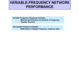
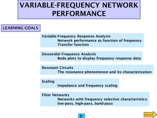
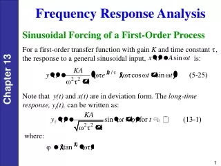
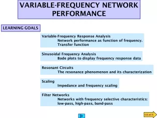
VARIABLE-FREQUENCY NETWORK PERFORMANCE LEARNING GOALS Variable-Frequency Response Analysis Network performance as function of frequency. Transfer function Sinusoidal Frequency Analysis Bode plots to display frequency response data Resonant Circuits The resonance phenomenon and its characterization Scaling Impedance and frequency scaling Filter Networks Networks with frequency selective characteristics: low-pass, high-pass, band-pass
Resistor VARIABLE FREQUENCY-RESPONSE ANALYSIS In AC steady state analysis the frequency is assumed constant (e.g., 60Hz). Here we consider the frequency as a variable and examine how the performance varies with the frequency. Variation in impedance of basic components
Simplified notation for basic components For all cases seen, and all cases to be studied, the impedance is of the form LEARNING EXAMPLE Moreover, if the circuit elements (L,R,C, dependent sources) are real then the expression for any voltage or current will also be a rational function in s MATLAB can be effectively used to compute frequency response characteristics
MATLAB commands required to display magnitude and phase as function of frequency EXAMPLE Missing coefficients must be entered as zeros This sequence will also work. Must be careful not to insert blanks elsewhere » num=[15*2.53*1e-3 0]; » den=[0.1*2.53*1e-3 15*2.53*1e-3 1]; » freqs(num,den) USING MATLAB TO COMPUTE MAGNITUDE AND PHASE INFORMATION NOTE: Instead of comma (,) one can use space to separate numbers in the array » num=[15*2.53*1e-3,0]; » den=[0.1*2.53*1e-3,15*2.53*1e-3,1]; » freqs(num,den)
GRAPHIC OUTPUT PRODUCED BY MATLAB Log-log plot Semi-log plot
LEARNING EXAMPLE A possible stereo amplifier Desired frequency characteristic (flat between 50Hz and 15KHz) Log frequency scale Postulated amplifier
Frequency Analysis of Amplifier Voltage Gain Frequency domain equivalent circuit required actual Frequency dependent behavior is caused by reactive elements
EXAMPLE Some nomenclature NETWORK FUNCTIONS When voltages and currents are defined at different terminal pairs we define the ratios as Transfer Functions If voltage and current are defined at the same terminals we define Driving Point Impedance/Admittance To compute the transfer functions one must solve the circuit. Any valid technique is acceptable
LEARNING EXAMPLE The textbook uses mesh analysis. We will use Thevenin’s theorem
EXAMPLE (More nomenclature) POLES AND ZEROS Arbitrary network function Using the roots, every (monic) polynomial can be expressed as a product of first order terms The network function is uniquely determined by its poles and zeros and its value at some other value of s (to compute the gain)
LEARNING EXTENSION Find the driving point impedance at Replace numerical values
Zeros = roots of numerator Poles = roots of denominator For this case the gain was shown to be Variable Frequency Response LEARNING EXTENSION
SINUSOIDAL FREQUENCY ANALYSIS Circuit represented by network function
By extension HISTORY OF THE DECIBEL Originated as a measure of relative (radio) power Using log scales the frequency characteristics of network functions have simple asymptotic behavior. The asymptotes can be used as reasonable and efficient approximations
Poles/zeros at the origin Frequency independent First order terms Quadratic terms for complex conjugate poles/zeros General form of a network function showing basic terms Display each basic term separately and add the results to obtain final answer Let’s examine each basic term
Constant Term Poles/Zeros at the origin
Simple pole or zero Asymptote for phase High freq. asymptote Behavior in the neighborhood of the corner Low freq. Asym.
Simple zero Simple pole
Magnitude for quadratic pole Phase for quadratic pole Quadratic pole or zero Corner/break frequency Resonance frequency These graphs are inverted for a zero
Generate magnitude and phase plots LEARNING EXAMPLE Draw asymptotes for each term Draw composites
Generate magnitude and phase plots LEARNING EXAMPLE Draw asymptotes for each Form composites
Final results . . . And an extra hint on poles at the origin
Sketch the magnitude characteristic LEARNING EXTENSION We need to show about 4 decades Put in standard form
Sketch the magnitude characteristic LEARNING EXTENSION Once each term is drawn we form the composites
Sketch the magnitude characteristic LEARNING EXTENSION Put in standard form Once each term is drawn we form the composites
LEARNING EXAMPLE A function with complex conjugate poles Put in standard form Draw composite asymptote Behavior close to corner of conjugate pole/zero is too dependent on damping ratio. Computer evaluation is better
Evaluation of frequency response using MATLAB Using default options » num=[25,0]; %define numerator polynomial » den=conv([1,0.5],[1,4,100]) %use CONV for polynomial multiplication den = 1.0000 4.5000 102.0000 50.0000 » freqs(num,den)
Evaluation of frequency response using MATLAB User controlled >> clear all; close all %clear workspace and close any open figure >> figure(1) %open one figure window (not STRICTLY necessary) >> w=logspace(-1,3,200);%define x-axis, [10^{-1} - 10^3], 200pts total >> G=25*j*w./((j*w+0.5).*((j*w).^2+4*j*w+100)); %compute transfer function >> subplot(211) %divide figure in two. This is top part >> semilogx(w,20*log10(abs(G))); %put magnitude here >> grid %put a grid and give proper title and labels >> ylabel('|G(j\omega)|(dB)'), title('Bode Plot: Magnitude response')
Compare with default! Evaluation of frequency response using MATLAB User controlled Continued USE TO ZOOM IN A SPECIFIC REGION OF INTEREST Repeat for phase >> semilogx(w,unwrap(angle(G)*180/pi)) %unwrap avoids jumps from +180 to -180 >> grid, ylabel('Angle H(j\omega)(\circ)'), xlabel('\omega (rad/s)') >> title('Bode Plot: Phase Response') No xlabel here to avoid clutter
LEARNING EXTENSION Sketch the magnitude characteristic
» num=0.2*[1,1]; » den=conv([1,0],[1/144,1/36,1]); » freqs(num,den)
A B C D E DETERMINING THE TRANSFER FUNCTION FROM THE BODE PLOT This is the inverse problem of determining frequency characteristics. We will use only the composite asymptotes plot of the magnitude to postulate a transfer function. The slopes will provide information on the order A. different from 0dB. There is a constant Ko B. Simple pole at 0.1 C. Simple zero at 0.5 D. Simple pole at 3 E. Simple pole at 20 If the slope is -40dB we assume double real pole. Unless we are given more data
C E A B Sinusoidal Determine a transfer function from the composite magnitude asymptotes plot LEARNING EXTENSION A. Pole at the origin. Crosses 0dB line at 5 B. Zero at 5 D C. Pole at 20 D. Zero at 50 E. Pole at 100
RESONANT CIRCUITS - SERIES RESONANCE QUALITY FACTOR RESONANT FREQUENCY PHASOR DIAGRAM
RESONANT CIRCUITS These are circuits with very special frequency characteristics… And resonance is a very important physical phenomenon The frequency at which the circuit becomes purely resistive is called the resonance frequency
Properties of resonant circuits At resonance the impedance/admittance is minimal Current through the serial circuit/ voltage across the parallel circuit can become very large (if resistance is small) Given the similarities between series and parallel resonant circuits, we will focus on serial circuits
Phasor diagram for series circuit Phasor diagram for parallel circuit Properties of resonant circuits At resonance the power factor is unity
Determine the resonant frequency, the voltage across each element at resonance and the value of the quality factor LEARNING EXAMPLE
Given L = 0.02H with a Q factor of 200, determine the capacitor necessary to form a circuit resonant at 1000Hz LEARNING EXAMPLE What is the rating for the capacitor if the circuit is tested with a 10V supply? The reactive power on the capacitor exceeds 12kVA
LEARNING EXTENSION Find the value of C that will place the circuit in resonance at 1800rad/sec Find the Q for the network and the magnitude of the voltage across the capacitor
Capacitor and inductor exchange stored energy. When one is at maximum the other is at zero The Q factor dissipates Stores as E field Stores as M field Q can also be interpreted from an energy point of view
ENERGY TRANSFER IN RESONANT CIRCUITS Normalization factor
Evaluated with EXCEL LEARNING EXAMPLE Determine the resonant frequency, quality factor and bandwidth when R=2 and when R=0.2
A series RLC circuit as the following properties: LEARNING EXTENSION Determine the values of L,C. 1. Given resonant frequency and bandwidth determine Q. 2. Given R, resonant frequency and Q determine L, C.
dependent For example LEARNING EXAMPLE Find R, L, C so that the circuit operates as a band-pass filter with center frequency of 1000rad/s and bandwidth of 100rad/s Strategy: 1. Determine Q 2. Use value of resonant frequency and Q to set up two equations in the three unknowns 3. Assign a value to one of the unknowns