Download
1 / 56
560 likes | 693 Views
Geology 510 Computer Aided Subsurface Interpretation Fall 2013. Everyday experience with spectra. Star light. http://www.arm.ac.uk/~csj/pus/spectra/tot_l.html. http://www.arm.ac.uk/~csj/pus/spectra/tot_l.html. Stellar emission spectra for individual atoms. From Wikipedia.

E N D
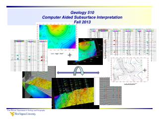
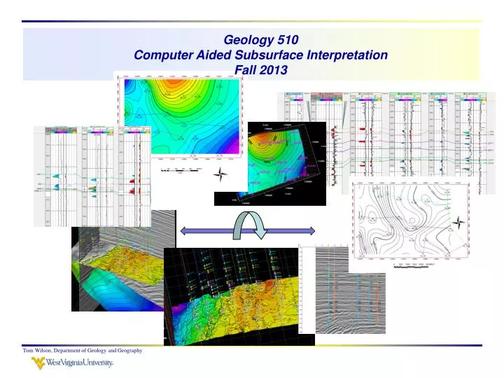
Geology 510Computer Aided Subsurface InterpretationFall 2013 Tom Wilson, Department of Geology and Geography
Everyday experience with spectra Tom Wilson, Department of Geology and Geography
Star light http://www.arm.ac.uk/~csj/pus/spectra/tot_l.html Tom Wilson, Department of Geology and Geography
http://www.arm.ac.uk/~csj/pus/spectra/tot_l.html Tom Wilson, Department of Geology and Geography
Stellar emission spectra for individual atoms From Wikipedia Tom Wilson, Department of Geology and Geography
We also encounter very interesting optical spectra applications in remote sensing Hyperspectral sensor collects data in 224 contiguous bands with 0.10 m bandwidths over the 0.4 to 2.5 m range. Tom Wilson, Department of Geology and Geography
Hydrothermal alteration at Cupritean RGB display comprised of 3 optical wavelengths Tom Wilson, Department of Geology and Geography
Wavelengths are chosen in areas that show some separation between the mineral components Tom Wilson, Department of Geology and Geography
RGB view and single frequency cube Tom Wilson, Department of Geology and Geography
Sunspot cycles in time and frequency Tom Wilson, Department of Geology and Geography
We talked briefly early on about spectral properties of Oxygen isotope concentrations Spectral peaks reveal different orbital components
Another example: Filtering out short wavelength features in a sonic log This log is from Marshall Co and penetrates the Pennsylvanian coal section and Mississippian A low pass filter Tom Wilson, Department of Geology and Geography
We’ve used frequency content to tell us something about Sooner D sand thickness and distribution Tom Wilson, Department of Geology and Geography
Some theory - long time window view of the seismic response in time and frequency Some useful references – Partyka, G., Gridley, J.,and Lopez, J., 1999, Interpretational application of spectral decomposition in reservoir characterization: The Leading Edge, 353-360. Partyka, G., Bottjer, R., and Peyton, L., 1998, Interpretation of incised valleys using new 3D techniques: a case history using spectral decomposition and coherency: The Leading Edge, 1294-1298. http://www.freeusp.org/RaceCarWebsite/TechTransfer/OnlineTraining/Spec_Tutorial/SpecDoc.html Tom Wilson, Department of Geology and Geography
Short window responses • In the shorter time window the reflection coefficient series is no longer randomly distributed or approximately random in distribution (not flat and featureless). • That is the same as saying that the geologic layering is not randomly distributed over short time or spatial windows. • Thus the local geology contributes significantly to the properties of the amplitude spectrum. Tom Wilson, Department of Geology and Geography
Cyclical geology produces an interference pattern in the amplitude spectrum Geology is not random – even over large time intervals. The geology often leaves an imprint on the amplitude spectrum. Tom Wilson, Department of Geology and Geography
The signal spectrum is a product of the spectra of the geology and the wavelet (plus some noise). Where the geology is represented by the reflection coefficient distribution R(f) in the small time window will usually produce a bumpy looking spectrum. Tom Wilson, Department of Geology and Geography
Long time window view of the seismic response in time and frequency So that the spectrum of the geology (the reflectivity is not featureless as shown here Partyka et al. (1999) Tom Wilson, Department of Geology and Geography
Local non-random reflectivity produces rippling in the spectrum Partyka et al. (1999) Tom Wilson, Department of Geology and Geography
Hence, as noted in the Sooner dataset, we often see a complex rippled spectrum The notches occur at about 10-11Hz intervals. Tom Wilson, Department of Geology and Geography
The spectrum in this 0.2 second long window The notches occur at about 30 Hz intervals. Tom Wilson, Department of Geology and Geography
The period of the notching is related to the time intervals between reflection events in your spectral window not just the thin bed reflection event Partyka et al. (1999) Tom Wilson, Department of Geology and Geography
Here’s some theory behind the relationship-The Fourier transform of thin bed reflectivity R The thin-bed reflectivity distribution to -to to is actually the one-way temporal thickness -R This t=2to The Fourier transform of r(t) = Tom Wilson, Department of Geology and Geography
The temporal thickness of the D Sand in the Sooner 3D is /2 or 0.008 seconds /2 the “temporal thickness” is the two way time through a layer at tuning. Tom Wilson, Department of Geology and Geography
Bring up tuning.xls and experiment What happens as the tuning thickness increases Here, a layer with two way time /2 of 0.016 seconds produces notches at 62.5 Hz. intervals in the spectrum. Tom Wilson, Department of Geology and Geography
Increased two-way times between the prominent reflections in your analysis window Brings spectral notches closer together Here the notches occur at 31.25 Hz. intervals. Tom Wilson, Department of Geology and Geography
Look at the spectrum on the far right Note that in our example, the period of notching (1/temporal thickness) equals 31.25 Hz. (1/0.032) Partyka et al. (1999) Tom Wilson, Department of Geology and Geography
Carry that over to a multi-trace representation of the thin bed response shown below Partyka et al. (1999) Tom Wilson, Department of Geology and Geography
Example spectrum from the Sooner 3D The notches occur at about 30 Hz intervals and imply that a layer with temporal thickness (on average) of about 33ms is prominent in the time window. Let’s assume that the real target of our exploration was a 20 foot thick sand with an interval velocity of 9500 ft/sec. Tom Wilson, Department of Geology and Geography
Some examples from the literature • The purpose of spectral decomposition is to see the seismic response at different, discrete frequency intervals, as the higher frequencies image thinner beds, while lower frequencies image thicker beds. • Spectral decomposition reveals details that no single frequency attribute can match. • Avoid choosing harmonics – you might try picking octave frequencies (the literature seemed a little unclear on this). VanDyke (2010) Tom Wilson, Department of Geology and Geography
How do you pick the frequencies to show in an RGB display If multiple channels or channel morphology produce channel segments that fall into two thickness categories then choose frequencies based on interval velocities for those possibilities VanDyke (2010) Tom Wilson, Department of Geology and Geography
Interpretation of incised valleys • Spectral decomposition and coherency have been shown to enhance interpretation of stratigraphic features in Tertiary, poorly lithified rocks, but their use has not been as well documented on older, more consolidated sediments. • Peyton et al. (1999) illustrate uses of spec decomp to image deep Pennsylvanian aged stratigraphic features in the mid-continent Anadarko Basin. • The example comes from the Upper Ref Fork incised valleys – noted as the largest and most clearly imaged valleys and also the best reservoir rocks in the area. Peyton et al. (1998) Tom Wilson, Department of Geology and Geography
Seismic data • The seismic data in the area consist of three surveys collected at different times • They were merged into a 136 mi2 data set. Merging usually involves some reprocessing to standardize the frequency content and wavelet phase. • Interpretation of the Red Fork incised valley using traditional interpretation techniques (autopicking, amplitude mapping, isochron mapping, etc.) did not provide clear reservoir views From Peyton et al. (1998) Tom Wilson, Department of Geology and Geography
Channel zone beneath the L. Skinnerin vertical section view From Peyton et al. (1998) Tom Wilson, Department of Geology and Geography
Interpreted Three different stages of valley fill From Peyton et al. (1998) Tom Wilson, Department of Geology and Geography
Spectral decomposition design • The authors note that the entire Red Fork sequence is about 50 ms thick • This was used to define the width of the design window ( the interval between the Lower Skinner and the Novi. From Peyton et al. (1998) Tom Wilson, Department of Geology and Geography
A frequency scan is often useful • Peyton et al. obtained good channel images in the 20 to 50 Hz. range and felt that the 36Hz amplitude slice provided optimal resolution. From Peyton et al. (1998) Tom Wilson, Department of Geology and Geography
Interpreted view • Peyton et al. obtained good channel images in the 20 to 50 Hz. range and felt that the 36Hz amplitude slice provided optimal resolution. From Peyton et al. (1998) Tom Wilson, Department of Geology and Geography
Outgrowths • The analysis helped establish an interconnection between producing Stage III wells in the west with those in the east. However a younger Stage V channel cuts through the Stage III channel diminishing prospect potential in that area. From Peyton et al. (1998) Tom Wilson, Department of Geology and Geography
Coherency view Coherency proved unable to resolve the Stage V channel, but did provide nice images of earlier channel complexes. Coherency also does not resolve internal channel detail obtained from in the spectral decomposition view. From Peyton et al. (1998) Tom Wilson, Department of Geology and Geography
The Stage V channel is unproductive and limited the extent of Stage III production The stage V channel turned out to be shale filled From Peyton et al. (1998) Tom Wilson, Department of Geology and Geography
Peyton et al. conclude Both spectral decomposition and coherency images show many valley-shaped features throughout the 3-D area in the Red Fork interval. Many of these features were previously unknown, and more work is needed to determine how they fit into the interpretation of the Red Fork. Well logs were critical to the interpretation. Coherency also led to the interpretation of valley-edge slump features and the recognition that not all faults in this area are basement involved. From Peyton et al. (1998) Tom Wilson, Department of Geology and Geography
Conventional energy envelope From Partyka et al. (1999) Tom Wilson, Department of Geology and Geography
16 Hz From Partyka et al. (1999) Tom Wilson, Department of Geology and Geography
26Hz From Partyka et al. (1999) Tom Wilson, Department of Geology and Geography
Phase spectra • Amplitude spectra delineate thin bed variability via spectral notching. • Phase spectra delineate lateral discontinuities via phase instability. From Partyka et al. (1999) Tom Wilson, Department of Geology and Geography
Phase at Frequency of 16 Hz From Partyka et al. (1999) Tom Wilson, Department of Geology and Geography
Phase at frequency of 26Hz From Partyka et al. (1999) Tom Wilson, Department of Geology and Geography
Partyka concludes • Real seismic is rarely dominated by simple blocky, resolved reflections. • In addition, true geologic boundaries rarely fall along fully resolved seismic peaks and troughs. • By transforming the data into the frequency domain with the discrete Fourier transform, short-window amplitude and phase spectra localize thin-bed reflections and define bed thickness variability within complex rock strata. • This allows the interpreter to quickly and effectively quantify thin-bed interference and detect subtle discontinuities within large 3-D surveys. Tom Wilson, Department of Geology and Geography
Isoproportional Slicing between horizons Tom Wilson, Department of Geology and Geography