Download
1 / 56
580 likes | 732 Views
Geology 510 Computer Aided Subsurface Interpretation Fall 2013. Objectives for the day. Spectral Analysis (see Monday) Convolutional model Wavelets Amplitude spectra Resolution and Synthetics. Frequency comparisons. Frequency comparisons. Log response.

E N D
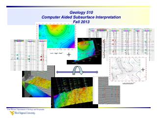
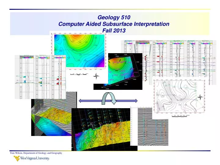
Geology 510Computer Aided Subsurface InterpretationFall 2013 Tom Wilson, Department of Geology and Geography
Objectives for the day • Spectral Analysis (see Monday) • Convolutional model • Wavelets • Amplitude spectra • Resolution and • Synthetics Tom Wilson, Department of Geology and Geography
Frequency comparisons Tom Wilson, Department of Geology and Geography
Frequency comparisons Tom Wilson, Department of Geology and Geography
Log response Tom Wilson, Department of Geology and Geography
Frequency versus peak-to-trough time Tom Wilson, Department of Geology and Geography
Program errorNote normal display can be QC’d using mouse and message bar at base of window Note value of 2.57 Tom Wilson, Department of Geology and Geography
Reverse values in color bar editor window. These changes carry over to the color bar in the display, but do not change colors of the map. The result as read from the color bar suggests P-T OWT time of ~1.45, while the mouse tip read out at the base reveals a value of ~2.57 Tom Wilson, Department of Geology and Geography
Acquisition footprint in the Sooner 3D observed using average energy attribute Tom Wilson, Department of Geology and Geography
Bring up the Sooner 3D and have a look at log settings Change color to cyan Width to 0.04 Tom Wilson, Department of Geology and Geography
Sonic is displayed with minimum (faster) to the rightthere are three wells with sonic near this line Tom Wilson, Department of Geology and Geography
Well locations Fed Sooner 7-21 has DT and RhoB Sooner unit 21-5-9 (DT and RhoB) Sooner unit 5-21 (DT and RhoB) Cross line 110 Tom Wilson, Department of Geology and Geography
Go to Tools > Generate Wavelet >Extract wavelet from seismic traces Extract wavelet from seismic traces Tom Wilson, Department of Geology and Geography
Tell kingdom how you want to estimate the waveletin this case from traces near a well Tom Wilson, Department of Geology and Geography
Select the Federal Sooner 7:21 and use a search radius of 250 feet Select a time window from t= 1.1 to 1.9 seconds Tom Wilson, Department of Geology and Geography
The wavelet window will pop up Tom Wilson, Department of Geology and Geography
Adjust the length to 0.2 seconds and click the compute spectrum button Tom Wilson, Department of Geology and Geography
Note spectral content and click on properties Set resolution to 10 Hz, start value to 0 and end value to 100 Tom Wilson, Department of Geology and Geography
This gives you a nice expanded view of the spectrum (total, signal and noise) Note that the bandwidth is approximately 15 to 78 Hz. Tom Wilson, Department of Geology and Geography
Change the sample interval to 0.0001 and next Tom Wilson, Department of Geology and Geography
Give the wavelet a name and finish Tom Wilson, Department of Geology and Geography
The wavelet is a critical component of the seismic response The wavelet shape can be thought of as the response of an isolated reflector. The wavelet Constructive interference From subsurfwiki.org The wavelet Tom Wilson, Department of Geology and Geography
Next let’s take a closer look at spectral content The spectrum has high amplitudes over a range extending from approximately 15 to 78 Hz. This is the spectrum of the wavelet we just created near the Federal Sooner well Tom Wilson, Department of Geology and Geography
We can also examine spectral properties for a variety of window sizes using Tom Wilson, Department of Geology and Geography
Here we define a range of lines and cross lines along with the time window as shown Here is our resulting spectrum Tom Wilson, Department of Geology and Geography
Recall that the D Sand is pronounced around instantaneous frequencies of about 50 to 60 Hz. Tom Wilson, Department of Geology and Geography
Note also that time slice in map display appears in your VuPak window Tom Wilson, Department of Geology and Geography
Here we’ve used a shorter time window Tom Wilson, Department of Geology and Geography
Note that in the time window surrounding the D Sand that there is a peak in the spectrum around 50 to 70 Hz. Tom Wilson, Department of Geology and Geography
Since reflectivity distribution often has an influence on wavelet shape we often compute a theoretical wavelet to use in the computation of a synthetic seismogram To do this, return to Tools > Generate wavelet > compute a theoretical wavelet Tom Wilson, Department of Geology and Geography
Use the Butterworth option Use the parameters below > next Tom Wilson, Department of Geology and Geography
Give it a name Tom Wilson, Department of Geology and Geography
Next – generate a synthetic for the Federal Sooner 7-21 well Tom Wilson, Department of Geology and Geography
Select the well > OK Tom Wilson, Department of Geology and Geography
T-D Chart > Velocity > Density …make your selections Tom Wilson, Department of Geology and Geography
Reference log, wavelet … Tom Wilson, Department of Geology and Geography
Trace > Extract trace > nearest Tom Wilson, Department of Geology and Geography
View and save extracted trace Tom Wilson, Department of Geology and Geography
Select that trace and Apply Tom Wilson, Department of Geology and Geography
Edit the display options (click the scale bar upper left) Tom Wilson, Department of Geology and Geography
Here is your synthetic Tom Wilson, Department of Geology and Geography
It’s pretty good, but it looks like the average velocity down to about 5500 feet is a little slow We can adjust this by shifting the synthetic upwards Tom Wilson, Department of Geology and Geography
Activate the shifter and click on the synthetic and drag up Tom Wilson, Department of Geology and Geography
Pin it and note that the positive cycle associated with the D Sand comes in a little early. pin shift Tom Wilson, Department of Geology and Geography
Shift that down and pin it Again, a pretty good match. It doesn’t always work out quite this well! Tom Wilson, Department of Geology and Geography
Zoom in on the bottom of the syntheticNote top and bottom of D Sand You can click on the esc key to deactivate the pin The read on depths to top and base of D Sand on the GR and /or AI curves extends ~ from 6354 to 6387 Tom Wilson, Department of Geology and Geography
Exit the synthetic and save Tom Wilson, Department of Geology and Geography
Lets look at the logs Tom Wilson, Department of Geology and Geography
View logs and change range (RC > Properties) 6352 6386 Tom Wilson, Department of Geology and Geography
You might want to adjust the picks on the top and base of the D Sand. Tops>edit formation tops Tom Wilson, Department of Geology and Geography