Download

1 / 45
450 likes | 606 Views
Introduction to Linkage and Association for Quantitative Traits. Michael C Neale Boulder Colorado Workshop March 2 2009. Overview. A brief history of SEM Regression Maximum likelihood estimation Models Twin data Sib pair linkage analysis Association analysis. Origins of SEM.

E N D
Introduction to Linkage and Association for Quantitative Traits Michael C Neale Boulder Colorado Workshop March 2 2009
Overview • A brief history of SEM • Regression • Maximum likelihood estimation • Models • Twin data • Sib pair linkage analysis • Association analysis
Origins of SEM • Regression analysis • ‘Reversion’ Galton 1877: Biological phenomenon • Yule 1897 Pearson 1903: General Statistical Context • Initially Gaussian X and Y; Fisher 1922 Y|X • Path Analysis • Sewall Wright 1918; 1921 • Path Diagrams of regression and covariance relationships
Structural Equation Modeling Basics • Two kinds of relationships • Linear regression X -> Y single-headed • Unspecified covariance X<->Y double-headed • Four kinds of variable • Squares: observed variables • Circles: latent, not observed variables • Triangles: constant (zero variance) for specifying means • Diamonds: observed variables used as moderators (on paths)
Linear Regression Covariance SEM Var(X) Res(Y) b Y X Models covariances only Of historical interest
Linear Regression SEM with means Var(X) Res(Y) b Y X M u(x) M u(y*) 1 Models Means and Covariances
Linear Regression SEM: Individual-level Yi = a + bXi Res(Y) X i b D Yi 1 a 1 Models Mean and Covariance of Y only Must have raw (individual level) data Xi is a definition variable Mean of Y different for every observation
1.00 F lm l1 l2 l3 S1 S2 S3 Sm e1 e2 e3 e4 Single Factor Covariance Model
Two Factor Model with Covs & Means 1 1.00 1.00 mF1 mF2 F1 F2 lm l3 l1 l2 S1 S2 S3 Sm mSm e1 e2 e3 e4 mS2 mS3 mS1 N.B. Not identified 1
Factor model essentials • In SEM the factors are typically assumed to be normally distributed • May have more than one latent factor • The error variance is typically assumed to be normal as well • May be applied to binary or ordinal data • Threshold model
Multifactorial Threshold Model Normal distribution of liability. ‘Affected’ when liability x > t t 0.5 0.4 0.3 0.2 0.1 0 -4 -3 -2 -1 0 1 2 3 4 x
Measuring Variation • Distribution • Population • Sample • Observed measures • Probability density function ‘pdf’ • Smoothed out histogram • f(x) >= 0 for all x
1 coin: 2 outcomes 2 coins: 3 outcomes Probability Probability 0.6 0.6 0.5 0.5 0.4 0.4 0.3 0.3 0.2 0.2 8 coins: 9 outcomes 0.1 0.1 Probability 0.3 0.25 0.2 0 0 0.15 HH Heads HT/TH Tails TT 0.1 0.05 0 Outcome Outcome Outcome Flipping Coins 4 coins: 5 outcomes Probability 0.4 0.3 0.2 0.1 0 HHHH HHHT HHTT HTTT TTTT Outcome
Bank of China Coin Toss Infinite outcomes 0.5 0.4 0.3 0.2 0.1 0 -4 -3 -2 -1 0 1 2 3 4 Heads-Tails De Moivre 1733 Gauss 1827
Variance: Average squared deviation Normal distribution xi di -3 -2 -1 0 1 2 3 Variance =di2/N
Deviations in two dimensions x + + + + + + + + + + + + + + y + + + + + + + + + + + + + + + + + + +
Deviations in two dimensions: dx x dy x dx + dy y
Covariance • Measure of association between two variables • Closely related to variance • Useful to partition variance • “Analysis of Variance” term coined by Fisher
Variance covariance matrix Univariate Twin/Sib Data Var(Twin1) Cov(Twin1,Twin2) Cov(Twin2,Twin1) Var(Twin2) Suitable for modeling when no missing data Good conceptual perspective
Maximum Likelihood Estimates: Nice Properties 1. Asymptotically unbiased • Large sample estimate of p -> population value 2. Minimum variance “Efficient” • Smallest variance of all estimates with property 1 3. Functionally invariant • If g(a) is one-to-one function of parameter a • and MLE (a) = a* • then MLE g(a) = g(a*) • See http://wikipedia.org
Full Information Maximum Likelihood (FIML) Calculate height of curve for each raw data vector -1
Height of normal curve:x = 0 Probability density function x (xi) -3 -2 -1 0 1 2 3 xi (xi) is the likelihood of data point xi for particular mean & variance estimates
Height of normal curve at xi:x = .5 Function of mean x (xi) -3 -2 -1 0 1 2 3 xi Likelihood of data point xi increases as x approaches xi
Likelihood of xi as a function of Likelihood function L(xi) MLE ^ -3 -2 -1 0 1 2 3 xi x L(xi) is the likelihood of data point xi for particular mean & variance estimates
Height of normal curve at x1 Function of variance x (xi var = 1) (xi var = 2) (xi var = 3) xi -3 -2 -1 0 1 2 3 Likelihood of data point xi changes as variance of distribution changes
Height of normal curve at x1 and x2 x (x1 var = 1) (x1 var = 2) (x2 var = 2) (x2 var = 1) x1 x2 -3 -2 -1 0 1 2 3 x1 has higher likelihood with var=1 whereas x2 has higher likelihood with var=2
0.5 0.4 0.3 3 2 1 0 -3 -2 -1 -1 0 -2 1 -3 2 3 Height of bivariate normal density function Likelihood varies as f( 1, 2, y x
Likelihood of Independent Observations • Chance of getting two heads • L(x1…xn) = Product (L(x1), L(x2) , … L(xn)) • L(xi) typically < 1 • Avoid vanishing L(x1…xn) • Computationally convenient log-likelihood • ln (a * b) = ln(a) + ln(b) • Minimization more manageable than maximization • Minimize -2 ln(L)
Likelihood Ratio Tests • Comparison of likelihoods • Consider ratio L(data,model 1) / L(data, model 2) • ln(a/b) = ln(a) - ln(b) • Log-likelihood lnL(data, model 1) - ln L(data, model 2) • Useful asymptotic feature when model 2 is a submodel of model 1 -2 (lnL(data, model 1) - lnL(data, model 2)) ~ df = # parameters of model 1 - # parameters of model 2 • BEWARE of gotchas! • Estimates of a2 q2 etc. have implicit bound of zero • Distributed as 50:50 mixture of 0 and -3 -2 -1 0 1 2 3 l
Two Group ACE Model for twin data 1 1(MZ) .5(DZ) 1 1 1 1 1 1 E C A A C E e c a a c e PT1 PT2 m m 1
Linkage Family-based Matching/ethnicity generally unimportant Few markers for genome coverage (300-400 STRs) Can be weak design Good for initial detection; poor for fine-mapping Powerful for rare variants Association Families or unrelated individuals Matching/ethnicity crucial Many markers req for genome coverage (105 – 106 SNPs) Powerful design Ok for initial detection; good for fine-mapping Powerful for common variants; rare variants generally impossible Linkage vs Association
Identity by Descent (IBD) Number of alleles shared IBD at a locus, parents AB and CD: Three subgroups of sibpairs AC AD BC BD AC 2 1 1 0 AD 1 2 0 1 BC 1 0 2 1 BD 0 1 1 2
Partitioned Twin Analysis • Nance & Neale (1989) Behav Genet 19:1 • Separate DZ pairs into subgroups • IBD=0 IBD=1 IBD=2 • Correlate Q with 0 .5 and 1 coefficients • Compute statistical power
Partitioned Twin Analysis: Three DZ groups .5 .25 1 .5 IBD=1 group A1 C1 D1 E1 Q1 Q2 E2 D2 C2 A2 P1 P2 IBD=2 group IBD=0 group 1 0 .25 1 .5 .25 1 .5 A1 C1 D1 E1 Q1 Q2 E2 D2 C2 A2 A1 C1 D1 E1 Q1 Q2 E2 D2 C2 A2 P1 P2 P1 P2
Problem 1 with Partitioned Twin analysis: Low Power • Power is low
Problem 2: IBD is not known with certainty • Markers may not be fully informative • Only so much heterozygosity in e.g., 20 allele microsatellite marker • Less in a SNP • Unlikely to have typed the exact locus we are looking for • Genome is big!
IBD pairs vary in similarity Effect of selecting concordant pairs IBD=2 t IBD=1 IBD=0 t
Improving Power for Linkage • Increase marker density (yaay SNP chips) • Change design • Families • Larger Sibships • Selected samples • Multivariate data • More heritable traits with less error
Problem 2: IBD is not known with certainty • Markers may not be fully informative • Only so much heterozygosity in e.g., 20 allele microsatellite marker • Less in a SNP • Unlikely to have typed the locus that causes variation • Genome is big! • The Universe is Big. Really big. It may seem like a long way to the corner chemist, but compared to the Universe, that's peanuts. - D. Adams
Using Merlin/Genehunter etc • Several Faculty experts • Goncalo Abecasis • Sarah Medland • Stacey Cherny • Possible to use Merlin via Mx GUI
“Pi-hat” approach 1 Pick a putative QTL location 2 Compute p(IBD=0) p(IBD=1) p(IBD=2) given marker data [Use Mapmaker/sibs or Merlin] 3 Compute i = p(IBD=2) + .5p(IBD=1) 4 Fit model Repeat 1-4 as necessary for different locations across genome ^ Elston & Stewart
Basic Linkage (QTL) Model i = p(IBDi=2) + .5 p(IBDi=1) individual-level 1 1 1 1 1 1 1 Pihat E1 F1 Q1 Q2 F2 E2 e f q q f e P1 P2 Q: QTL Additive Genetic F: Family Environment E: Random Environment3 estimated parameters: q, f and e Every sibship may have different model P P
Association Model 1 Geno1 Geno2 LDL1i= a + b Geno1i Var(LDLi) = R Cov(LDL1,LDL2) = C C may be f(i) in joint linkage & association G2 G1 b a a b LDL1 LDL2 C R R
Between/Within Fulker Association Model M Geno1 Geno2 Model for the means G1 G2 0.50 LDL1i = .5bGeno1 + .5bGeno2 + .5wGeno1 - .5wGeno2 = .5( b(Geno1+Geno2) + w(Geno1-Geno2) ) 0.50 -0.50 0.50 S D m m b w B W 1.00 1.00 -1.00 1.00 LDL1 LDL2 R R C