Download
1 / 58
590 likes | 755 Views
Genetic principles for linkage and association analyses. Manuel Ferreira & Pak Sham. Boulder, 2009. Gene mapping. LOCALIZE and then IDENTIFY a locus that regulates a trait. Association analysis. Linkage analysis. Linkage:.

E N D
Genetic principles for linkage and association analyses Manuel Ferreira & Pak Sham Boulder, 2009
Gene mapping LOCALIZE and then IDENTIFY a locusthat regulates a trait Association analysis Linkage analysis
Linkage: If a locus regulates a trait, Trait Varianceand Covariance between individuals will be influenced by this locus. Association: If a locus regulates a trait, Trait Mean in the population will also be influenced by this locus.
Revisit common genetic parameters - such as allele frequencies, genetic effects, dominance, variance components, etc Use these parameters to construct a biometric genetic model • Model that expresses the: • Mean • Variance • Covariance between individuals • for a quantitative phenotype as a function of the genetic parameters of a given locus. See how the biometric model provides a useful framework for linkage and association methods.
Outline 1. Genetic concepts 2. Very basic statistical concepts 3. Biometrical model 4. Introduction to linkage analysis
A. DNA level DNA structure, organization recombination G G G G G G B. Population level G G G Allele and genotype frequencies G G G G G G G G G G G C. Transmission level G G Mendelian segregation Genetic relatedness G G D. Phenotype level Biometrical model P P Additive and dominance components
A. DNA level A DNA molecule is a linear backbone of alternating sugar residues and phosphate groups Attached to carbon atom 1’ of each sugar is a nitrogenous base: A, C, G or T Two DNA molecules are held together in anti-parallel fashion by hydrogen bonds between bases [Watson-Crick rules] Antiparallel double helix A gene is a segment of DNA which is transcribed to give a protein or RNA product Only one strand is read during gene transcription Nucleotide: 1 phosphate group + 1 sugar + 1 base
DNA polymorphisms Microsatellites >100,000 Many alleles, eg. (CA)n repeats, very informative SNPs 14,708,752 (build 129, 03 Mar ‘09) Most with 2 alleles (up to 4), not very informative A Copy Number Variants >5,000 Many alleles, just recently automated B
DNA organization 22 + 1 2 (22 + 1) 2 (22 + 1) 2 (22 + 1) ♂ ♁ ♂ A - A - A - ♁ B - ♂ ♁ ♁ ♂ Mitosis B - B - chr1 A - A - A - - A A - - A ♁ ♁ ♂ B - B - B - - B B - - B A - - A - A B - - B - B chr1 G1 phase S phase M phase Haploid gametes Diploid zygote 1 cell Diploid zygote >1 cell
DNA recombination 22 + 1 22 + 1 A - NR (♂) B - A - - A chr1 2 (22 + 1) 2 (22 + 1) B - - B - A ♁ Meiosis R chr1 (♂) (♁) ♂ ♁ - B A - A - - A - A chr1 B - B - - B - B A - R chr1 chr1 chr1 chr1 (♁) A - - A B - chr1 Diploid gamete precursor cell B - - B - A chr1 NR - B Haploid gamete precursors chr1 Hap. gametes
DNA recombination between linked loci 22 + 1 A - NR B - (♂) A - - A B - - B 2 (22 + 1) - A ♁ Meiosis NR - B (♂) (♁) ♂ ♁ A - A - - A - A B - B - - B - B A - NR B - (♁) A - - A B - - B Diploid gamete precursor - A - B NR Haploid gamete precursors Hap. gametes
B. Population level 1. Allele frequencies A single locus, with two alleles - Biallelic - Single nucleotide polymorphism, SNP A a a a a A a a A A A a A a Alleles A and a - Frequency of A is p - Frequency of a is q = 1 – p A A A A A a A a A A A a a A genotype is the combination of the two alleles A a Aa
B. Population level 2. Genotype frequencies (Random mating) Allele 1 A (p) a (q) A (p) AA (p2) Aa (pq) Allele 2 a (q) aa (q2) aA (qp) Hardy-Weinberg Equilibrium frequencies P (AA) = p2 P (Aa) = 2pq p2+ 2pq + q2 = 1 P (aa) = q2
C. Transmission level Mendel’s law of segregation Mother (A3A4) Segregation (Meiosis) Gametes A3(½) A4(½) A1(½) A1A3(¼) A1A4(¼) Father (A1A2) A2(½) A2A4(¼) A2A3(¼)
D. Phenotype level 1. Classical Mendelian traits Dominant trait - AA, Aa1 - aa0 Huntington’s disease (CAG)n repeat, huntingtin gene Recessive trait - AA 1 - aa, Aa0 Cystic fibrosis 3 bp deletion exon 10 CFTR gene
AA Aa aa D. Phenotype level 2. Quantitative traits e.g. cholesterol levels
D. Phenotype level Aa P(X) aa AA X aa Aa AA m
D. Phenotype level Aa P(X) Biometric Model aa AA X aa Aa AA m +a d – a Genotypic effect
Mean, variance, covariance 1. Mean (X)
Mean, variance, covariance 2. Variance (X)
Mean, variance, covariance 3. Covariance (X,Y)
Biometrical model for single biallelic QTL Biallelic locus - Genotypes: AA, Aa, aa - Genotype frequencies: p2, 2pq, q2 Alleles at this locus are transmitted from P-O according to Mendel’s law of segregation Genotypes for this locus influence the expression of a quantitative trait X (i.e. locus is a QTL) Biometrical genetic modelthat estimates the contribution of this QTL towards the (1) Mean, (2) Variance and (3) Covariancebetween individuals for this quantitative trait X
Biometrical model for single biallelic QTL 1. Contribution of the QTL to the Mean (X) e.g. cholesterol levels in the population Genotypes Aa aa AA a d -a Effect, x p2 2pq q2 Frequencies, f(x) Mean (X) = a(p2) + d(2pq) – a(q2) = a(p-q) + 2pqd
Biometrical model for single biallelic QTL 2. Contribution of the QTL to the Variance (X) Genotypes Aa aa AA a d -a Effect, x p2 2pq q2 Frequencies, f(x) Var (X) = (a-m)2p2 + (d-m)22pq + (-a-m)2q2 = VQTL Heritability of X at this locus = VQTL/ V Total
Biometrical model for single biallelic QTL Var (X) = (a-m)2p2 + (d-m)22pq + (-a-m)2q2 =2pq[a+(q-p)d]2 + (2pqd)2 m = a(p-q) + 2pqd = VAQTL+ VDQTL Additive effects: the main effects of individual alleles Dominance effects: represent the interaction between alleles
Biometrical model for single biallelic QTL d = 0 (no dominance) d +a – a +a +a m = 0 aa Aa AA Additive model
Biometrical model for single biallelic QTL d > 0 (dominance) d +a – a +a+d +a-d m = 0 aa Aa AA Dominant model
Biometrical model for single biallelic QTL d < 0 (dominance) d +a – a +a-d +a+d m = 0 aa Aa AA Recessive model
Statistical definition of dominance is scale dependent +4 +4 +0.7 +0.4 log (x) aa AA aa AA Aa Aa No departure from additivity Significant departure from additivity
Biometrical model for single biallelic QTL a 0 Genotypic mean -a aa AA aa AA aa AA aa AA Aa Aa Aa Aa Additive Dominant Recessive Var (X) = Regression Variance + Residual Variance = Additive Variance + Dominance Variance = VAQTL+ VDQTL
Practical H:\manuel\biometric\sgene.exe
Practical Aim Visualize graphically how allele frequencies, genetic effects, dominance, etc, influence trait mean and variance Ex1 a=0, d=0, p=0.4, Residual Variance = 0.04, Scale = 2. Vary a from 0 to 1. Ex2 a=1, d=0, p=0.4, Residual Variance = 0.04, Scale = 2. Vary d from -1 to 1. Ex3 a=1, d=0, p=0.4, Residual Variance = 0.04, Scale = 2. Vary p from 0 to 1. Look at scatter-plot, histogram and variance components.
Some conclusions • Additive genetic variance depends on allele frequency p & additive genetic value a as well as dominance deviation d • Additive genetic variance typically greater than dominance variance
Biometrical model for single biallelic QTL 1. Contribution of the QTL to the Mean (X) 2. Contribution of the QTL to the Variance (X) 3. Contribution of the QTL to the Covariance (X,Y)
Biometrical model for single biallelic QTL 3. Contribution of the QTL to the Cov (X,Y) (a-m) Aa aa (-a-m) (d-m) AA (a-m)2 (a-m) AA (d-m) (a-m) (d-m) (d-m)2 Aa aa (-a-m)2 (-a-m) (-a-m) (d-m) (-a-m) (a-m)
Biometrical model for single biallelic QTL 3A. Contribution of the QTL to the Cov (X,Y) – MZ twins (a-m) Aa aa (-a-m) (d-m) AA p2 (a-m)2 (a-m) AA (d-m) (a-m) (d-m) (d-m)2 Aa 0 2pq aa (-a-m)2 (-a-m) (-a-m) (d-m) (-a-m) q2 0 (a-m) 0 Cov(X,Y) = (a-m)2p2 + (d-m)22pq + (-a-m)2q2 = VAQTL+ VDQTL =2pq[a+(q-p)d]2 + (2pqd)2
Biometrical model for single biallelic QTL 3B. Contribution of the QTL to the Cov (X,Y) – Parent-Offspring (a-m) Aa aa (-a-m) (d-m) AA p3 (a-m)2 (a-m) AA (d-m) (a-m) (d-m) (d-m)2 Aa p2q pq aa (-a-m)2 (-a-m) (-a-m) (d-m) (-a-m) q3 0 (a-m) pq2
e.g. given an AAfather, an AAoffspring can come from either AAx AAor AAx Aaparental mating types AAx AA will occur p2× p2 = p4 and have AA offspring Prob()=1 AAx Aa will occur p2× 2pq = 2p3q and have AA offspring Prob()=0.5 and have Aa offspring Prob()=0.5 Therefore, P(AA father & AAoffspring) = p4 + p3q = p3(p+q) = p3
Biometrical model for single biallelic QTL 3B. Contribution of the QTL to the Cov (X,Y) – Parent-Offspring (a-m) Aa aa (-a-m) (d-m) AA p3 (a-m)2 (a-m) AA (d-m) (a-m) (d-m) (d-m)2 Aa p2q pq aa (-a-m)2 (-a-m) (-a-m) (d-m) (-a-m) q3 0 (a-m) pq2 Cov (X,Y) = (a-m)2p3 + … + (-a-m)2q3 = ½VAQTL =pq[a+(q-p)d]2
Biometrical model for single biallelic QTL 3C. Contribution of the QTL to the Cov (X,Y) – Unrelated individuals (a-m) Aa aa (-a-m) (d-m) AA p4 (a-m)2 (a-m) AA (d-m) (a-m) (d-m) (d-m)2 Aa 2p3q 4p2q2 aa (-a-m)2 (-a-m) (-a-m) (d-m) (-a-m) q4 p2q2 (a-m) 2pq3 Cov (X,Y) = (a-m)2p4 + … + (-a-m)2q4 = 0
Biometrical model for single biallelic QTL 3D. Contribution of the QTL to the Cov (X,Y) – DZ twins and full sibs ¼ genome ¼ genome ¼ genome ¼ genome # identical alleles inherited from parents 2 1 (father) 0 1 (mother) ¼ (2 alleles) + ½ (1 allele) + ¼ (0 alleles) Unrelateds MZ twins P-O Cov (X,Y) = ¼ Cov(MZ) + ½ Cov(P-O) + ¼ Cov(Unrel) = ¼(VAQTL+VDQTL) + ½ (½ VAQTL) + ¼ (0) = ½ VAQTL + ¼VDQTL
Biometrical model predicts contribution of a QTL to the mean, variance and covariances of a trait Association analysis = a(p-q) + 2pqd Mean (X) Linkage analysis = VAQTL+ VDQTL Var (X) = VAQTL+ VDQTL Cov (MZ) On average! = ½VAQTL+ ¼VDQTL Cov (DZ) For a given locus, do two sibs have 0, 1 or 2 alleles in common? 0, 1/2 or 1 0 or 1 IBD estimation / Linkage
For a heritable trait... Linkage: localize region of the genome where a QTL that regulates the trait is likely to be harboured Family-specific phenomenon: Affected individuals in a family share the same ancestral predisposing DNA segment at a given QTL Can only detect very large effects Association: identify a QTL that regulates the trait Population-specific phenomenon: Affected individuals in a population share the same predisposing DNA segment at a given QTL Can detect weaker effects
Controls Cases Families No Linkage No Association Linkage No Association Linkage Association
Non-parametric linkage approach Linkage tests co-segregation between a marker and a trait If a trait locus truly regulates the expression of a phenotype, then two relatives with similar phenotypes should have inherited from a common ancestor the same predisposing allele at a marker near the trait locus, and vice-versa. Interest: correlation between phenotypic similarity and genetic similarity at a locus