Download
1 / 46
470 likes | 618 Views
Linkage and association. Sarah Medland. Genotypic similarity between relatives. IBS Alleles shared Identical By State “look the same”, may have the same DNA sequence but they are not necessarily derived from a known common ancestor - focus for association. M 3. M 1. M 2. M 3. Q 3.

E N D
Linkage and association Sarah Medland
Genotypic similarity between relatives IBSAlleles shared Identical By State “look the same”, may have the same DNA sequence but they are not necessarily derived from a known common ancestor - focus for association M3 M1 M2 M3 Q3 Q1 Q2 Q4 IBDAlleles shared Identical By Descent are a copy of the same ancestor allele - focus for linkage M1 M2 M3 M3 Q1 Q2 Q3 Q4 IBD IBS M1 M3 M1 M3 2 1 Q1 Q4 Q1 Q3
In linkage analysis we will be estimating an additional variance component Q • For each locus under analysis the coefficient of sharing for this parameter will vary for each pair of siblings • The coefficient will be the probability that the pair of siblings have both inherited the same alleles from a common ancestor
MZ=1.0 DZ=0.5 MZ & DZ = 1.0 1 1 1 1 1 1 1 1 Q A C E E C A Q e c a q q a c e PTwin1 PTwin2
Alternative approach • is a summary statistic • Convenient • Loss of information • .5 can mean p.ibd0=0 p.ibd1=1 p.ibd2=0 or p.ibd0=0 p.ibd1=.6 p.ibd2=.2 • Use all the information
Alternative approach • Model each of the possible outcomes • IBD0 IBD1 IBD2 • Weight each of the models by the probability that it is the correct model • The pairwise likelihood is equal to the sum of likelihood for each model multiplied by the probability it is the correct model • The combined likelihood is equal to the sum of all the pairwise likelihoods
DZ pairs * pIBD2 + * pIBD1 + * pIBD0
How to do this in mx? Tells Mx we will be using 3 different means and variance models • Script link_mix.mx G2 DZ TWINS Data NInput=124 NModel=3 Missing =-99.00 Rectangular File=example3.dat Labels …. Select pheno1 pheno2 z0_20 z1_20 z2_20 age1 sex1 age2 sex2; Definition_variables z0_20 z1_20 z2_20 age1 sex1 age2 sex2; Tells Mx that these variables will be used as covariates – the values for these variables will be updated for each case during the optimization – the mxo will show the values for the final case
How to do this in mx? This script runs an AE model D is the QTL VC path coefficent Begin Matrices; X Lower nvar nvar = X1 Z Lower nvar nvar = Z1 D Lower nvar nvar = D1 B full 3 1 ! will contain IBD probabilities (from Genehunter) def var … Matrix H 0.5 Specify B z0_20 z1_20 z2_20 ! put ibd probabilities in B We are placing the prob. Of being IBD 0 1 & 2 in the B matrix
How to do this in mx? Pre-computing the total variance and the covariance for the diff. IBD groups Begin Algebra; T = X*X'+Z*Z'+D*D' ; ! total variance U = H@X*X' ; ! IBD 0 cov (=non-qtl cov) K = U + H@D*D' ; ! IBD 1 cov W = U + D*D' ; ! IBD 2 cov A = T|U_ U|T_ ! IBD 0 matrix T|K_ K|T_ ! IBD 1 matrix T|W_ W|T ; ! IBD 2 matrix Stacking the pre-computed covariance matrices
How to do this in mx? The means matrix contains corrections for age and sex – it is repeated 3 times and vertically stacked Means G+O*R'| G+S*R'_G+O*R'| G+S*R'_G+O*R'| G+S*R'; Covariance A ; Weights B ; Tells Mx to weight each of the means and var/cov matrices by the IBD prob. which we placed in the B matrix
Summary • Weighted likelihood approach more powerful than pi-hat • Quickly becomes unfeasible • 3 models for sibship size 2 • 27 models for sibship size 4 • Q: How many models for sibship size 3? • For larger sib-ships/arbitrary pedigrees pi-hat approach is method of choice
Association Introduction
Association • Simplest design possible Correlate phenotype with genotype • Candidate genes for specific diseases common practice in medicine/genetics • Genome-wide association with millions available SNPs, can search whole genome exhaustively
Allelic Association SNPs trait variant chromosome Genetic variation yields phenotypic variation More copies of ‘B’ allele More copies of ‘b’ allele
2a Genotype Genetic Value BB Bb bb a d -a Biometrical model d bb midpoint Bb BB Va (QTL) = 2pqa2 (no dominance)
Basic premise of assoc. for qualitative trait • Chose a phenotype & a candidate gene(s) • Collect 2 groups - cases and controls • Unrelated individuals • Matched for relevant covariates • Genotype your individuals for your gene(s) • Count the % of cases & controls with each genotype • Run a chi-square test 0 1
The equivalent for a quantitative trait- run a regression Yi = a + bXi + ei where Yi = trait value for individual i Xi = 1 if allele individual i has allele ‘A’ 0 otherwise i.e., test of mean differences between ‘A’ and ‘not-A’ individuals Play with Association.xls 0 1
Practical – Find a gene for sensation seeking: • Two populations (A & B) of 100 individuals in which sensation seeking was measured • In population A, gene X (alleles 1 & 2) does not influence sensation seeking • In population B, gene X (alleles 1 & 2) does not influence sensation seeking • Mean sensation seeking score of population A is 90 • Mean sensation seeking score of population B is 110 • Frequencies of allele 1 & 2 in population A are .1 & .9 • Frequencies of allele 1 & 2 in population B are .5 & .5
.01 .18 .81 .25 .50 .25 Genotypic freq. Sensation seeking score is the same across genotypes, within each population. Population B scores higher than population A Differences in genotypic frequencies
Suppose we are unaware of these two populations and have measured 200 individuals and typed gene X The mean sensation seeking score of this mixed population is 100 What are our observed genotypic frequencies and means? Calculating genotypic frequencies in the mixed population Genotype 11: 1 individual from population A, 25 individuals from population B on a total of 200 individuals: (1+25)/200=.13 Genotype 12: (18+50)/200=.34 Genotype 22: (81+25)/200=.53 Calculating genotypic means in the mixed population Genotype 11: 1 individual from population A with a mean of 90, 25 individuals from population B with a mean of 110 = ((1*90) + (25*110))/26 =109.2 Genotype 12: ((18*90) + (50*110))/68 = 104.7 Genotype 22: ((81*90) + (25*110))/106 = 94.7
Genotypic freq. .13 .34 .53 Gene X is the gene for sensation seeking! Now, allele 1 is associated with higher sensation seeking scores, while in both populations A and B, the gene was not associated with sensation seeking scores… FALSE ASSOCIATION
.01 .18 .81 .25 .50 .25 Genotypic freq. What if there is true association? allele 1 frequency 0.5 allele 2 frequency 0.5. allele 1 = -2 allele 2 = +2 Pop mean = 110 allele 1 frequency 0.1 allele 2 frequency 0.9 allele 1 = -2, allele 2 = +2 Pop mean = 90
Calculate: • Genotypic means in mixed population • Genotypic frequencies in mixed population • Is there an association between the gene and sensation seeking score? If yes which allele is the increaser allele?
Dm = Difference in subpopulation mean =-10 5 Overestimation 4 =-5 3 Genuine allelic effect=+2 2 Estimated value of allelic effect Underestimation 1 0 =5 -1 Reversal effects -2 =10 -3 0.49 0.42 0.35 0.28 0.07 0.00 -0.07 -0.28 -0.35 -0.42 -0.49 0.21 0.14 -0.14 -0.21 Differencein gene frequency in subpopulations False positives and false negatives Posthuma et al., Behav Genet, 2004
How to avoid spurious association? True association is detected in people coming from the same genetic stratum • Can check that individuals come from the same population using a large set of highly polymorphic genes – genomic control • Can use family members as controls – family based association
Fulker (1999) between/within association model Fulker et al, AJHG, 1999
bij as Family Control • bij is the expected genotype for each individual • Ancestors • Siblings • wij is the deviation of each individual from this expectation • Informative individuals • To be “informative” an individual’s genotype should differ from expected • Have heterozygous ancestor in pedigree • βb≠ βw is a test for population stratification • βw > 0 is a test for association free from stratification
So… • 4 tests for the price of one • Test for pop-stratification aw=ab • Robust test for association aw=0 • Test so see if linked loci is the functional variant QTL≠ 0 in the presence of aw it is in LD with the variant but is not the casual variant • Test for dominance effects if dominance is also modeled
Combined Linkage & associationImplemented in QTDT (Abecasis et al., 2000) and Mx (Posthuma et al., 2004) • Association and Linkage modeled simultaneously: • Association is modeled in the means • Linkage is modeled in the (co)variances • QTDT: simple, quick, straightforward, but not so flexible in terms of models • Mx: less simple, but highly flexible
Implementation in Mx link_assoc.mx #define n 3 ! number of alleles is 3, coded 1, 2, 3 … G1: calculation group between and within effects Data Calc Begin matrices; A Full 1 n free ! additive allelic effects within C Full 1 n free ! additive allelic effects between D Sdiag n n free ! dominance deviations within F Sdiag n n free ! dominance deviations between I Unit 1 n ! one's End matrices; Specify A 100 101 102 Specify C 200 201 202 Specify D 800 801 802 Specify F 900 901 902 The locus has 3 alleles These 1*3 vector matrices contain the b/n & w/n additive effects of each of the 3 alleles These 3*3 off-diagonal matrices contain the b/n & w/n dominance effects of each of the 3 alleles
Sticking it together… Begin algebra; K = (A'@I) + (A@I') ; ! Within effects, additive L = D + D' ; ! Within effects, dominance W = K+L ; ! Within effects - additive and dominance in one matrix M = (C'@I) + (C@I') ; ! Between effects, additive N = F + F' ; ! Between effects, dominance B = M+N ; ! Between effects - additive and dominance in one matrix End algebra ;
W = K+L ; This is the 1/2 genotype mean composed of the simple additive effects of allele 1 + allele 2 and any deviation from these simple additive effects (dominance effects) K+L =
W = K+L ; K+L (parameter numbers) = Between effects stick together in the same way
I = [ 1 1 1], A = [a1 a2 a3] D = 0 0 0 d21 0 0 d31 d32 0 K = (A'@I) + (A@I') = a1 1 a2 @ [1 1 1] + [a1 a2 a3] @ 1 = a3 1 a1 a1 a1 a1 a2 a3 a1a1 a1a2 a1a3 a2 a2 a2 + a1 a2 a3 = a2a1 a2a2 a2a3 a3 a3 a3 a1 a2 a3 a3a1 a3a2 a3a3 L = D + D' = 0 0 0 0 d21 d31 0 d21 d31 d21 0 0 + 0 0 d32 = d21 0 d32 d31 d32 0 0 0 0 d31 d32 0 W = K+L = a1a1 a1a2 a1a3 0 d21 d31 a1a1 a1a2d21 a1a3d31 a2a1 a2a2 a2a3 + d21 0 d32 = a2a1d21 a2a2 a2a3d32 a3a1 a3a2 a3a3 d31 d32 0 a3a1d31 a3a2d32 a3a3 K = (A'@I) + (A@I') ; ! Within effects, additive L = D + D' ; ! Within effects, dominance W = K+L ; ! Within effects total M = (C'@I) + (C@I') ; ! Between effects, additive N = F + F' ; ! Between effects, dominance B = M+N ; ! Between effects - total
B = c1c1c1c2f21 c1c3f31 c2c1f21 c2c2 c2c3f32 c3c1f31 c3c2f32 c3c3 W = a1a1a1a2d21 a1a3d31 a2a1d21 a2a2 a2a3d32 a3a1d31 a3a2d32 a3a3 • We have a sibpair with genotypes 1,1 and 1,2. μ1 = Grand mean + pair mean + ½ pair difference μ2 = Grand mean + pair mean - ½ pair difference • To calculate the between-pairs effect, or the mean genotypic effect of this pair, we need matrix B: ((c1c1) + (c1c2f21)) / 2 • To calculate the within-pair effect we need matrix W and the between pairs effect: For sib1: (a1a1) + ((c1c1) + (c1c2f21)) / 2 For sib2: (a1a2d21) - ((c1c1) + (c1c2f21)) / 2
G3: datagroup: sibship size two, DZ … Definition_variables tw1a1 tw1a2 tw2a1 tw2a2 … Begin Matrices; … G Full 1 nvar = G2 ! grand mean B Computed n n = B1 ! spurious and genuine genotypic effects (between) W Computed n n = W1 ! genuine genotypic effects (within) K Full 1 4 Fix ! Will contain first and second allele of twin1 L Full 1 4 Fix ! Will contain first and second allele of twin2 S Full 1 1 Fix ! Will contain 2 (for two individuals per family) … End Matrices; Matrix K 1 1 1 1 Matrix L 1 1 1 1 Specify K tw1a1 tw1a2 tw1a1 tw1a2 Specify L tw2a1 tw2a2 tw2a1 tw2a2 Alleles 1 and 2 for twins 1 and 2 respectively We are going to put the allele numbers here These matrices must be initialized –given default values Alleles 1 and 2 for twins 1 and 2 respectively
B = c1c1c1c2f21 c1c3f31 c2c1f21 c2c2 c2c3f32 c3c1f31 c3c2f32 c3c3 Sticking it together using part • For sibpairs 1,1 and 1,2 • To calculate the between-pairs effect, or the mean genotypic effect of this pair, we need matrix B: ((c1c1) + (c1c2f21)) / 2 • We can use the part function to draw out a specified element of a matrix
B = c1c1 c1c2f21 c1c3f31 c2c1f21 c2c2 c2c3f32 c3c1f31 c3c2f32 c3c3 Sticking it together using part • We can use the part function to draw out a specified element of a matrix • So to draw out c3c1f31 we could say: \part(B, K) where K is a matrix containing 1 3 1 3
B= c1c1 c1c2f21 c1c3f31 c2c1f21 c2c2 c2c3f32 c3c1f31 c3c2f32 c3c3 W = a1a1 a1a2d21 a1a3d31 a2a1d21 a2a2 a2a3d32 a3a1d31 a3a2d32 a3a3 Sibpair with genotypes: 1,1 and 1,2 Specify K tw1a1 tw1a2 tw1a1 tw1a2 = 1 1 1 1 Specify L tw2a1 tw2a2 tw2a1 tw2a2 = 1 2 1 2 V = (\part(B,K) + \part(B,L) ) %S ; (c1c1 + c1c2f21)/2 C = (\part(W,K) + \part(W,L) ) %S ; (a1a1 + a1a2d21)/2 Means G + F*R '+ V + (\part(W,K)-C) | G + I*R' + V +(\part(W,L)-C); = G + F*R’ + (c1c1 + c1c1f21)/2 + (a1a1 - (a1a1 + a1a2d21)/2)| G + I*R' + (c1c1 + c1c1f21)/2 + (a2a1 - (a1a1 + a1a2d21)/2)
Constrain sum additive allelic within effects = 0 Constraint ni=1 Begin Matrices; A full 1 n = A1 O zero 1 1 End Matrices; Begin algebra; B = \sum(A) ; End Algebra; Constraint O = B ; end Constrain sum additive allelic between effects = 0 Constraint ni=1 Begin Matrices; C full 1 n = C1 ! O zero 1 1 End Matrices; Begin algebra; B = \sum(C) ; End Algebra; Constraint O = B ; end
!1.test for linkage in presence of full association Drop D 2 1 1 end !2.Test for population stratification: !between effects = within effects. Specify 1 A 100 101 102 Specify 1 C 100 101 202 Specify 1 D 800 801 802 Specify 1 F 800 801 802 end !3.Test for presence of dominance Drop @0 800 801 802 end !4.Test for presence of full association Drop @0 800 801 802 100 101 end !5.Test for linkage in absence of association Free D 2 1 1 end