Download
1 / 54
540 likes | 544 Views
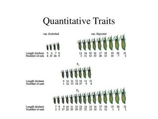
Basic Statistics for Linkage and Association Studies of Quantitative Traits. Boulder Colorado Workshop March 5 2007. Overview. A brief history of SEM Regression Maximum likelihood estimation Models Twin data Sib pair linkage analysis Association analysis Mixture distributions

E N D
Basic Statistics for Linkage and Association Studies of Quantitative Traits Boulder Colorado Workshop March 5 2007
Overview • A brief history of SEM • Regression • Maximum likelihood estimation • Models • Twin data • Sib pair linkage analysis • Association analysis • Mixture distributions • Some extensions
Origins of SEM • Regression analysis • ‘Reversion’ Galton 1877: Biological phenomenon • Yule 1897 Pearson 1903: General Statistical Context • Initially Gaussian X and Y; Fisher 1922 Y|X • Path Analysis • Sewall Wright 1918; 1921 • Path Diagrams of regression and covariance relationships
Structural Equation Model basics • Two kinds of relationships • Linear regression X -> Y single-headed • Unspecified covariance X<->Y double-headed • Four kinds of variable • Squares – observed variables • Circles – latent, not observed variables • Triangles – constant (zero variance) for specifying means • Diamonds -- observed variables used as moderators (on paths)
Linear Regression Model Var(X) Res(Y) b Y X Models covariances only Of historical interest
Linear Regression Model Var(X) Res(Y) b Y X Mu(x) Mu(y*) 1 Models Means and Covariances
Linear Regression Model Res(Y) X i b D Yi 1 Mu(y*) 1 Models Mean and Covariance of Y only Must have raw (individual level) data X is a definition variable Mean of Y different for every observation
1.00 F lm l1 l2 l3 S1 S2 S3 Sm e1 e2 e3 e4 Single Factor Model
Factor Model with Means MF 1.00 1.00 mF1 mF2 F1 F2 lm l1 l2 l3 S1 S2 S3 Sm mSm e1 e2 e3 e4 mS2 mS3 mS1 B8
Factor model essentials • The factor itself is typically assumed to be normally distributed: SEM • May have more than one latent factor • The error variance is typically assumed to be normal as well • May be applied to binary or ordinal data • Threshold model
Multifactorial Threshold Model Normal distribution of liability. ‘Affected’ when liability x > t t 0.5 0.4 0.3 0.2 0.1 0 -4 -3 -2 -1 0 1 2 3 4 x
Measuring Variation • Distribution • Population • Sample • Observed measures • Probability density function ‘pdf’ • Smoothed out histogram • f(x) >= 0 for all x
One Coin toss 2 outcomes Probability 0.6 0.5 0.4 0.3 0.2 0.1 0 Heads Tails Outcome
Two Coin toss 3 outcomes Probability 0.6 0.5 0.4 0.3 0.2 0.1 0 HH HT/TH TT Outcome
Four Coin toss 5 outcomes Probability 0.4 0.3 0.2 0.1 0 HHHH HHHT HHTT HTTT TTTT Outcome
Ten Coin toss 9 outcomes Probability 0.3 0.25 0.2 0.15 0.1 0.05 0 Outcome
Fort Knox Toss Infinite outcomes 0.5 0.4 0.3 0.2 0.1 0 -4 -3 -2 -1 0 1 2 3 4 Heads-Tails De Moivre 1733 Gauss 1827
Variance • Measure of Spread • Easily calculated • Individual differences
Average squared deviation Normal distribution xi di -3 -2 -1 0 1 2 3 Variance =di2/N
Measuring Variation Weighs & Means • Absolute differences? • Squared differences? • Absolute cubed? • Squared squared?
Measuring Variation Ways & Means • Squared differences Fisher (1922) Squared has minimum variance under normal distribution Concept of “Efficiency” emerges
Deviations in two dimensions x + + + + + + + + + + + + + + y + + + + + + + + + + + + + + + + + + +
Deviations in two dimensions x dx + dy y
Covariance • Measure of association between two variables • Closely related to variance • Useful to partition variance • Analysis of variance coined by Fisher
Summary Formulae for sample statistics; i=1…N observations x= (xi)/N x = (xi - x) / (N) 2 2 xy= (xi-x)(yi-y) / (N) r= xy xy 2 2 x x
Variance covariance matrix Univariate Twin/Sib Data Var(Twin1) Cov(Twin1,Twin2) Cov(Twin2,Twin1) Var(Twin2) Only suitable for complete data Good conceptual perspective
Summary • Means and covariances • Basic input statistics for “Traditional SEM” • Notion of probability density function
Maximum Likelihood Estimates: Nice Properties 1. Asymptotically unbiased • Large sample estimate of p -> population value 2. Minimum variance “Efficient” • Smallest variance of all estimates with property 1 3. Functionally invariant • If g(a) is one-to-one function of parameter a • and MLE (a) = a* • then MLE g(a) = g(a*) • See http://wikipedia.org
Likelihood computation Calculate height of curve -1
Height of normal curve: x = 0 Probability density function x (xi) -3 -2 -1 0 1 2 3 xi (xi) is the likelihood of data point xi for particular mean & variance estimates
Height of normal curve at xi: x = .5 Function of mean x (xi) -3 -2 -1 0 1 2 3 xi Likelihood of data point xi increases as x approaches xi
Height of normal curve at x1 Function of variance x (xi var = 1) (xi var = 2) (xi var = 3) x1 -3 -2 -1 0 1 2 3 Likelihood of data point xi changes as variance of distribution changes
Height of normal curve at x1 and x2 x (x1 var = 1) (x1 var = 2) (x2 var = 2) (x2 var = 1) x1 x2 -3 -2 -1 0 1 2 3 x1 has higher likelihood with var=1 whereas x2 has higher likelihood with var=2
Likelihood of xi as a function of Likelihood function L(xi) MLE ^ -3 -2 -1 0 1 2 3 xi x L(xi) is the likelihood of data point xi for particular mean & variance estimates
Likelihood as a measure of “outlierness” • Unlikely observation may be an outlier • Genuine • Data entry error • Model-specific • Can use Mx feature to obtain case-wise likelihoods • Raw data • Option mx%p= uni_pi.out • Output for each case: the contribution to the -2ll as well as z-score statistic and Mahalanobis distance, weight and weighted likelihood • Generates R syntax to read in file, and sort by z-score • Beeby Medland & Martin (2006) ViewPoint and ViewDist: utilities for rapid graphing of linkage distributions and identification of outliers. Behav Genet. 2006 Jan;36(1):7-11
0.5 0.4 0.3 3 2 1 0 -3 -2 -1 -1 0 -2 1 -3 2 3 Height of bivariate normal density function An unlikely pair of (x,y) values y y1 x x1
0.5 0.4 0.3 3 2 1 0 -3 -2 -1 -1 0 -2 1 -3 2 3 Height of bivariate normal density function A more likely pair of (x,y) values y2 x2
Likelihood of Independent Observations • Chance of getting two heads • L(x1…xn) = Product (L(x1), L(x2) , … L(xn)) • L(xi) typically < 1 • Avoid vanishing L(x1…xn) • Computationally convenient log-likelihood • ln (a * b) = ln(a) + ln(b) • Minimization more manageable than maximization • Minimize -2 ln(L)
Likelihood Ratio Tests • Comparison of likelihoods • Consider ratio L(data,model 1) / L(data, model 2) • Ln(a/b) = ln(a) - ln(b) • Log-likelihood lnL(data, model 1) - ln L(data, model 2) • Useful asymptotic feature when model 2 is a submodel of model 1 -2 (lnL(data, model 1) - lnL(data, model 2)) ~ df = # parameters of model 1 - # parameters of model 2 • BEWARE of gotchas! • Estimates of a2 q2 etc. have implicit bound of zero • Distributed as 50:50 mixture of 0 and -3 -2 -1 0 1 2 3 l
Exercises: Compute Normal PDF • Get used to Mx script language • Use matrix algebra • Taste of likelihood theory
Mx script part 1: Declare groups and matrices #NGroups 1 Title figure out likelihood by hand Calculation Begin Matrices; E symm 2 2 ! Expected Covariance Matrix H full 1 1 ! One half T full 1 1 ! Two M full 2 1 ! Mean vector P full 1 1 ! Pi X full 2 1 ! Observed Data End Matrices;
Mx script part 2: Put values in matrices Matrix E 1 .0 1 Matrix H .5 Matrix M 0 0 Matrix P 3.141592 Matrix T 2 Matrix X 1 2
Mx script part 3: Matrix Algebra Begin Algebra; O=T*P*\sqrt\det(E); ! Fractional part, 2pi*sqrt(det(e)) Q=(X-M)'&(E~); ! Mahalanobis Distance R=\exp(-H*Q); ! e to the power -.5*Mahalanobis distance S=-T*\ln(R%O);! minus twice log-likelihood Z=-T*\ln(\pdfnor(X'_M'_E)); ! A simpler way End Algebra; End Group;
Exercises 1 • Bivariate normal distribution • Means [110.28 112.00] • Covariance matrix [299.40 174.20 281.18] • Compute likelihood of observed vector x = [87 89]
Exercises 2 • Bivariate normal distribution • Means [1 1] • Covariance matrix [1 .3 .3 1 ] • Compute likelihood of observed vector x = [1 2] • Compute likelihood with correlation of .0 instead • Optional compute likelihood of observed vector x = [-2 -2] with correlations .5, .0, and 0 • Which is the most likely combination of model and data?
Exercises 3 • Univariate normal distribution • Mean [1] • Variance [1 ] • Compute likelihood of observed vector x = [1] • Compute likelihood of observed vector x = [2] • Compute their product • Which bivariate case does this equal?
Two Group Model: ACE MZ twins DZ twins 7 parameters
DZ by IBD status Variance = Q + F + E Covariance = πQ + F + E
Extensions to More Complex Applications • Endophenotypes • Linkage Analysis • Association Analysis
Basic Linkage (QTL) Model = p(IBD=2) + .5 p(IBD=1) 1 1 1 1 1 1 1 Pihat E1 F1 Q1 Q2 F2 E2 e f q q f e P1 P2 Q: QTL Additive Genetic F: Family Environment E: Random Environment3 estimated parameters: q, f and e Every sibship may have different model P P