Download
1 / 37
590 likes | 1.4k Views
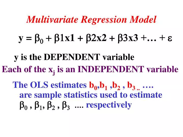
Multivariate Regression Model. y = b 0 + b1 x1 + b2 x2 + b3 x3 +… + e. The OLS estimates b 0 , b 1 , b 2 , b 3 .. …. are sample statistics used to estimate b 0 , b 1 , b 2 , b 3 .... respectively. y is the DEPENDENT variable. Each of the x j is an INDEPENDENT variable.

E N D
Multivariate Regression Model y = b0 + b1x1 + b2x2 + b3x3 +… + e The OLS estimates b0,b1 ,b2 , b3 .. …. are sample statistics used to estimate b0,b1, b2 , b3 .... respectively y is the DEPENDENT variable Each of the xj is an INDEPENDENT variable
Each explanatory variable Xj is assumed (1A) to be deterministic or non-random Conditions: (1B) : to come from a‘fixed’population (1C) : to have a variance V(xj) which is not ‘too large’ The above assumptions are best suited to a situation of a controlled experiment
Assumptions concerning the random term ei : (IIA) E(ei) = 0 for all i (IIB) Var(ei) = s2 = constant for all i (IIC) Covariance (ei , ek) = 0 for any i and k (IID) Each of the ei has a normal distribution
1. Each of these statistics is a linear functions of the Y values. Properties of b0 , b1 , b2 , b3 2. Therefore, they all have normal distributions 3. Each is an unbiased estimator. That is, E(bk) = bk;
4. Each bk is the most efficient estimator of all unbiased estimators.
Thus, each of b0 , b1 , b2 ….is Best Linear Unbiased Estimator of the respective parameter
Conclusion Each estimator bi has a normal distribution with mean = biand variance = bi2 where bi2 is unknown.
Income(£ per week) of an individual is regressed on a constant, education (in years), age (in years) and wealth inheritance(in £), using EViews. Number of observations is 20 and the regression output is given below:
Variable CoefficientStd.Errort-Stats Prob. C-1001.87520.71-1.920.0654 AGE8.855.451.620.1168 EDUCATION 95.1738.542.46 0.0252 WEALTH 1.510.463.26 0.0031
The Maximum Type 1 Error = Significance Level Significance Level (a)
p-value The smaller the p-value the more significant is the test
The proposed regression model is: Income = ß0 + ß1(Age) +ß2(Education) + ß3(Wealth Inheritance) … . .(A) We are proposing that Income is the variable dependent on three independent variables: Age, Education and Wealth.
It measures the effect of other deterministic factors on Income not included in the model. b0is a constant. b1, b2, b3measure the effect of a marginal change in Age, Education and Wealth, respectively.
However, we recognise that there may be other random factors affecting the dependent variable Income. So we add a random variable to the model which now becomes: Income = ß0 + ß1(Age) +ß2(Education) + ß3(Wealth Inherited) + … . . (B)
We use the least squares technique to estimate the model B. Therefore, our estimation of the proposed model B is Ye = -1001.87 + 8.85*AGE + 95.17*EDUCATION + 1.51*WEALTH INHERITANCE Here Yeis the estimated value of income
-1001.87 is the estimate of ß0, 8.85 is the estimate of ß1,; 95.17 is the estimate of ß2 and 1.51 is the estimate of ß3 The least-squares estimates of the ß-values are denoted by b-values. Thus, b1 is the estimate of ß1 and b2is the estimate of ß2 . In our case, b1 = 8.85 and b2 = 95.17.
We next make the following assumptions on the specification of model B so that the least-squares method produces ‘good’ estimators.
i. is normally distributed with mean 0 and an unknown variance 2 . In the context of the model B, can be thought of as a luck factor which can be good (positive values) or bad (negative values), If the positive and negative values cancel out on average, we can say that mean value is 0.
(Whether or not you are lucky does not influence my being lucky/unlucky) The values are uncorrelated across the population i. The values have the same variance (2) across it. (Every individual is exposed to the same extent/chance of good or bad luck)
The values are uncorrelated with the independent variables Age, Education and WealthInheritance. (For example, an old person is as likely to be lucky as a young one; or a university graduate is as likely to be unlucky as someone with no A-levels).
We now test (at 10% significance) the following hypothesis: Education has a positive effect on income Step 1: Set up the hypotheses H0 : ß2 = 0 (Educationhas no effect) H1 : ß2 > 0(Education has a positive effect) one-tailed test
Step 2: Select statistic The estimator b2 is the test-statistic Step3 : Identify the distribution of b2
Assumptions i-iii above imply that b2 is Best Linear in the dependent variable income Unbiased Estimator of 2
Since b2 is unbiased, E(b2) = 2 Thus, b2~ N(2, 22) where 22is unknown. b2 has a normal distribution because it is linear in Income
Step 4: Construct test statistic We use the standard error of b2 because we do not know what 22is Therefore, the test statistic is t (b2- 2) / (standard error of b2) has a Student’s t-distribution with 20-4 = 16 d.o.f.
As 2 = 0 under the null hypothesis (H0) t = b2 / (standard error of b2) EViews therefore gives us a t-statistic regarding education of 2.46907 The corresponding probability value is 0.0252.
Select fx /TDIST. For X, enter 2.469607, the t-Statistic value. The degree of freedom is 16. EViews calculates two-tail probability So number of tails is 2. You now get the 2-tail probability of 0.025165 from Excel. Since we are performing a one-tail test, take half the probability value, or 0.0126 .
Step 5: Compare with critical value tC tC = 1.336757 for a one-tailed test with significance level (a) = 0.1 and d.o.f. = 16 tC = 1.336757 < 2.469607
Step 6 : Draw conclusion The test is significant. Reject H0 at 10% and at 5% (1.745884 < 2.469607) but not at 1% (2.583492 > 2.469607) Step 7: Interpret result The data supports (with at least 98% accuracy) the hypothesis that EDUCATION is an important explanatory variable affecting income.
In rejecting H0, we are prone to make a Type 1 Error. The probability of a type 1 error is nothing but the area to the right of t-statistic, or 0.0126.
The Model :: y = a + bx + e and add the assumptions (Lec17) Example 2: Use output 2 to test the hypothesis (at 5% significance) that weightgain is proportional to foodvalue. Step 1: H0 : a= 0 (proportionality) H1 : a 0 (non-proportionality) Step 2: The estimator a is the test-statistic
The explanatory variable X is assumed (1A) to be deterministic or non-random Conditions: (1B) : to come from a‘fixed’population (1C) : to have a variance V(x) which is not ‘too large’ The above assumptions are best suited to a situation of a controlled experiment
Assumptions concerning the random term ei : (IIA) E(ei) = 0 for all i (IIB) Var(ei) = s2 = constant for all i (IIC) Covariance (ei , ej) = 0 for any i and j (IID) Each of the ei has a normal distribution
Step 3: Thus, a~ N(a, 2) where 2is unknown. Step 4: Therefore, the test statistic t (a- a) / (standard error of a) has a Student’s t-distribution with 10-2 = 8 d.o.f.
Step 5: Compare with critical value tC tC = -2.31 for a two-tailed test with significance level (a) = 0.05 and d.o.f.= 8 The p-value is 0.0169 < 0.05 Step 6: Draw conclusion The test is significant. Reject H0 at 5% tC = -2.31 > -3.005262 Step 7: Interpret Foodvalue is not the only variable that affects weightgain
Example 3: Use output 3 to test (at 5% significance) the following hypothesis: Exercise has a negative effect on weight gain The proposed regression model is: Weightgain = ß0 + ß1(Foodvalue) +ß2(Exercise) + e
Step 1: Set up the hypotheses H0 : ß2 = 0 (Exercisehas no effect) H1 : ß2 < 0(Exercise has a negative effect)