Multivariate Regression

Multivariate Regression

Topics • The form of the equation • Assumptions • Axis of evil (collinearity, heteroscedasticity and autocorrelation) • Model miss-specification • Missing a critical variable • Including irrelevant variable (s)

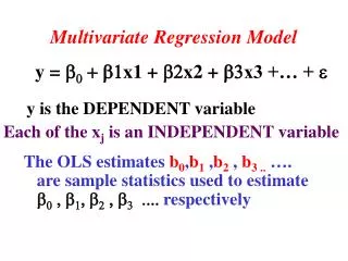
The form of the equation Yt= Dependent variable a1 = Intercept b2= Constant (partial regression coefficient) b3= Constant (partial regression coefficient) X2 = Explanatory variable X3 = Explanatory variable et = Error term

Partial Correlation (slope) Coefficients B2 measures the change in the mean value of Y per unit change in X2, while holding the value of X3 constant. (Known in calculus as a partial derivative) Y = a +bX dy = b

Assumptions of MVR • X2 and X3 are non-stochastic, that is, their values are fixed in repeated sampling • The error term e has a zero mean value (Σe/N=0) • Homoscedasticity, that is the variance of “e”, is constant. • No autocorrelation exists between the error term and the explanatory variable. • No exact collinearity exist between X2 and X3 • The error term “e” follows the normal distribution with mean zero and constant variance

Venn Diagram: Correlation & Coefficients of Determination (R2) Y Y X2 X1 X1 X2 Correlation exists between X1 and X2. There is a portion of the variation of Y that can be attributed to either one No correlation exists between X1 and X2. Each variable explains a portion of the variation of Y

A special case: Perfect Collinearity Y X1 X2 X2 is a perfect function of X1. Therefore, including X2 would be irrelevant because does not explain any of the variation on Y that is already accounted by X1. The model will not run.

Consequences of Collinearity Multicollinearity is related to sample-specific issues • Large variance and standard error of OLS estimators • Wider confidence intervals • Insignificant t ratios • A high R2 but few significant t ratios • OLS estimators and their standard error are very sensitive to small changes in the data; they tend to be unstable • Wrong signs of regression coefficients • Difficult to determine the contribution of explanatory variables to the R2

TESTING FOR MULTICOLLINEARITY

DEPENDENT TLA BATHS BEDROOM AGE

More on multicollinearity When VIF =1 there is zero multicollinearity, meaning that R2=0 Because VIF = 1/ (1 – R2 )

IS IT BAD, IF WE HAVE MULTICOLLINEARITY? • If the goal of the study is to use the model to predict or forecast the future mean value of the dependent variable, collinearity may not be a problem • If the goal of the study is not prediction but reliable estimation of the parameters then collinearity is a serious problem • Solutions: Dropping variables, acquire more data or a new sample, rethinking the model or transform the form of the variables.

Heteroscedasticity • Heteroscedasticity: The variance of “e” is not constant, therefore, violates the assumption of hemoscedasticity or equal variance.

Heteroscedasticity

What to do when the pattern is not clear ? • Run a regression where you regress the residuals or error term on Y.

LET’S ESTIMATE HETEROSCEDASTICITY Do a regression where the residuals become the dependent Variable and home value the independent variable.

Consequences of Heteroscedasticity • OLS estimators are still linear • OLS estimators are still unbiased • But they no longer have minimum variance. They are not longer BLUE • Therefore we run the risk of drawing wrong conclusions when doing hypothesis testing (Ho:b=0) • Solutions: variable transformation, develop a new model that takes into account no linearity (logarithmic function).

Testing for Heteroscedasticity Let’s regress the predicted value (Y hat) on the log of the residual (log e2) to see the pattern of heteroscedasticity. Log e2 The above pattern shows that our relationships is best described as a Logarithmic function

Autocorrelation • Time-series correlation: The best predictor of sales for the present Christmas season is the previous Christmas season • Spatial correlation: The best predictor of a home’s value is the value of a home next door or in the same area or neighborhood. • The best predictor for a politician, to win an election as an incumbent, is the previous election (ceteris paribus)

Autocorrelation • Gujarati defines autocorrelation as “correlation between members of observations ordered in time [as time- series data] or space as [in cross-sectional data]. E (UiUj)=0 The product of two different error terms Ui and Uj is zero. • Autocorrelation is a model specification error or the regression model is not specified correctly. A variable is missing or has the wrong functional form.

Types of Autocorrelation

The Durbin Watson Test (d) of Autocorrelation Values of the d d = 4 (perfect negative correlation d = 2 (no autocorrelation) d = 0 (perfect positive correlation)

Let’s do a “d” test Here we solved the problem of collinearity, heteroscedasticity and autocorrelation. It cannot get any better than this.

Model Miss-specification • Omitted variable bias or underfitting a model. Therefore • The omitted variable is correlated with the included variable then the parameters estimated are bias, that is their expected values do not match the true value • The error variance estimated is bias • The confidence intervals and hypothesis-testing procedures and unreliable. • The R2 is also unreliable • Let’s run a model (Olympic medals)

Model Miss-specification • Irrelevant variable bias • The unnecessary variables has not effect on Y (although R2may increase). • The model still give us unbias and consistent estimates of the coefficients • The major penalty is that the true parameters are less precise therefore the CI are wider increasing the risk of drawing invalid inference during hypothesis testing (accept the Ho: B=0) • Let’s run the following model:

Medals and Development

Missing a key variable

When a key variable is included

Did Mexico underperformed in the 2004 Summer Olympics? • Medals (4) • Inv rank (125) • Pop (98) Y (hat) = -7.219+.147(125)+.043(98) Y (hat) = 15.36

Even a better model

Thanks. The End

Multivariate Regression