Download
1 / 18
180 likes | 424 Views
More on Multivariate Regression Analysis. Multivariate F-Tests Multicolinearity The EVILS of Stepwise Regression Intercept Dummies Interaction Effects Interaction Dummies Slope Dummies. F-Tests.

E N D
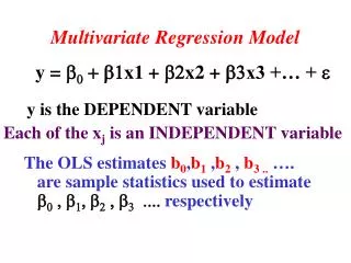
More on Multivariate Regression Analysis • Multivariate F-Tests • Multicolinearity • The EVILS of Stepwise Regression • Intercept Dummies • Interaction Effects • Interaction Dummies • Slope Dummies
F-Tests F-tests are used to test for the statistical significance of the overall model fit. Normally, that’s redundant given that you already have the t-stats for the individual b’s. This amounts to a ratio of the explained variance by the residual variance, correcting for the number of observations and parameters. The F value is compared to the F-distribution, just like a t-distribution, to obtain a p-value. F-tests become useful when we need to assess nested models.
F-Tests, continued The question is whether a more complex model adds to the explanatory power over a simpler model. E.g., using the Guns data, does including a set of gender/age (pm1024) and race (pb1064) variables improve the prediction of the violent crime rate (vio) variable after we’ve included average income (avginc) and population density (density)? To find out, we calculate an F-statistic for the model improvement: • Where the complex model has K parameters, and the simpler model has K-H parameters. • RSS{K-H} is the residual sum of squares for the simpler model • RSS{K} is the residual sum of squares for the more complex model
F-Testing a Nested Model Simpler Model: vio = b0 + b1(avginc) + b2(density) More Complex Model: vio = b0 + b1(avginc) + b2(density) + b3(pm1024) + b4(pb1064) Given the models, K = 5, K - H = 3, and n = 1173. Calculating the RSS’s involves running the two models, obtaining the RSS from each. For these models, RSSK = 60,820,479.3and RSSK-H = 68,295,254.4. So: Given that df1 = H (2) and df2 = n-K (1168), the p-value of the model improvement shown in Appendix Table 5C (p. 762) is <0.01.
In-Class Homework -- Set 1 • Test for the additional explanatory power of the age/gender and race varables (pm1024 and pb1064) when modeling the murder and robbery rates (mur and rob). Use the simple model from the prior lecture exercise (avginc and density) as your base of comparison. • Discuss the theoretical meaning of your results.
Multicolinearity • If any Xi is a linear combination of other X’s in the model, bi cannot be estimated • Remember that the partial regression coefficient strips both the X’s and Y of the overlapping covariation: • If an X is perfectly predicted by the other X’s, then:
Multicolinearity, Continued • We rarely find perfect multicolinearity in practice, but high multicolinearity results in loss of statistical resolution: • Large standard errors • Low t-stats, high p-values • Erodes hypothesis tests • Enormous sensitivity to small changes in: • Data • Model specification
Detecting Multicolinearity • Use of VIF measures: • Variance Inflation Factor • Degree to which other coefficients’ variance is increased due to the inclusion of the specified variable • 1/VIF is equivalent to: (AKA “Tolerance”) • Acceptable tolerance? Partly a function of n-size: • If n < 50, tolerance should exceed 0.7 • If n < 300, tolerance should exceed 0.5 • If n < 600, tolerance should exceed 0.3 • If n < 1000, tolerance should exceed 0.1 • Calculating Tolerance in Stata (using VIF)
Addressing Multicolinearity • Drop one or other of co-linear variables • Caution: May result in model mis-specification • Use theory as a guide • Add new data • Special samples may maximize independent variation • E.g.: Elite samples may disentangle income, education • Data Scaling • Highly correlated variables may represent multiple indicators of an underlying scale • Data reduction through factor analysis • More on this later
In-Class Homework: Set 2 • Run a VIF on the “more complex” model from the nested F-test exercise (from lecture slide #5) • Now add the variable pw1064 (percent of the population white, ages 10-64). Run VIF again. • Using the pm1024 and pb1064 variables • F-Test will show significant improvement (over the reduced model from earlier) • But not all individual coefficients were statistically significant • What gives? • Correlate pb1064, pw1064 and pm1029 • Strategy? • Drop either pw1064 or pb1064 (use theory to decide which) • Re-run the model
Evils of Mindless Regression • Stata permits a number of mechanical “search strategies” • Stepwise regression (forward, backward, upside down) • How they work: use of sequential F-tests • These methods pose serious problems: • If X’s are strongly related, one or the other will tend to be excluded • Susceptible to inclusion of spuriously related variables • Obliterates the meaning of classical statistical tests • Hypothesis tests depend on prior hypothesis identification • Example: The infamous Swedish “EMF study” • Hundreds of diseases regressed on proximity to EMF sources • about 5% found to be “statistically significant” • Enormous policy implications -- but method was buried in report
Dummy Intercept Variables • Dummy variables allow for tests of the differences in overall value of the Y for different nominal groups in the data (akin to a difference of means) • Coding: 0 and 1 values (e.g., men versus women) Y X2,0 X2,1 X1
Modeling Robbery as a function of Population Density and “Shall Issue” laws Source | SS df MS Number of obs = 1173 -------------+------------------------------ F( 2, 1170) = 983.14 Model | 21362735.3 2 10681367.7 Prob > F = 0.0000 Residual | 12711578.7 1170 10864.5972 R-squared = 0.6269 -------------+------------------------------ Adj R-squared = 0.6263 Total | 34074314 1172 29073.6468 Root MSE = 104.23 ------------------------------------------------------------------------------ rob | Coef. Std. Err. t P>|t| [95% Conf. Interval] -------------+---------------------------------------------------------------- density | 96.56459 2.2606 42.72 0.000 92.12931 100.9999 shall | -50.08407 7.141642 -7.01 0.000 -64.09593 -36.07221 _cons | 139.9945 3.635576 38.51 0.000 132.8616 147.1275 ------------------------------------------------------------------------------ Robbery rates are systematically lower in “Shall Issue” states (is this necessarily causal??)
Dummy Variable Applications • Implies a comparison (the omitted group) • Be clear about the “comparison category” • Multinomial Dummies • When categories exceed 2 • Importance of specifying the base category • Examples of Category Variables • Experimental treatment groups • Race and ethnicity • Region of residence • Type of education • Religious affiliation • “Seasonality” • Adds to modeling flexibility
Interaction Effects • Interactions occur when the effect of one X is dependent on the value of another • Modeling interactions: • Use Dummy variables (requires categories) • Use multiplicative interaction effect • Multiply an interval scale times a dummy (also known as a “slope dummy”) • Example: the effect of Population Density (density) on Robbery Rate (rob) may be affected by whether the respondent in in a Shall Issue state or not • Re-code the interaction; run it.
Modeling Robbery with a Dummy Slope Variable: Density * Shall Source | SS df MS Number of obs = 1173 -------------+------------------------------ F( 3, 1169) = 706.02 Model | 21956237.5 3 7318745.84 Prob > F = 0.0000 Residual | 12118076.5 1169 10366.1903 R-squared = 0.6444 -------------+------------------------------ Adj R-squared = 0.6435 Total | 34074314 1172 29073.6468 Root MSE = 101.81 ------------------------------------------------------------------------------ rob | Coef. Std. Err. t P>|t| [95% Conf. Interval] -------------+---------------------------------------------------------------- density | 96.13354 2.208874 43.52 0.000 91.79974 100.4673 shall | -103.8476 9.957383 -10.43 0.000 -123.3839 -84.31126 i | 648.0681 85.64837 7.57 0.000 480.0264 816.1098 _cons | 140.1835 3.551295 39.47 0.000 133.2159 147.1512 ------------------------------------------------------------------------------
Coming Up... • Assumptions of OLS Revisited • Visual Diagnostic Techniques • Non-linearity • Non-normality and Heteroscedasticity • Outliers and Case Statistics • Aren’t we having fun now?