Download
1 / 26
290 likes | 430 Views
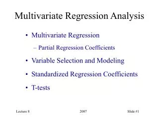
Multivariate Regression Analysis. Aim. Establish a predictive model between one or more response variables and one or more input variables. Measurement. Response. Areas where Regression Analysis is useful. Process and Environmental Monitoring Process Control

E N D
Aim • Establish a predictive model between one or more response variables and one or more input variables Measurement Response
Areas where Regression Analysis is useful • Process and Environmental Monitoring • Process Control • Product Quality/Product Properties
Why? • Reveal correspondences/correlations • Increased Accuracy/Precision in the Information Process • Improved (reduced) Response time in the Information Process (“on-line”, “at-line”)
How? 1. Collect Data 2. Analyse Data 3. Establish a Predictive Model Y = BX, yi = f (x1, x2, .., xm) y = bx, y = f (x1, x2, .., xm)
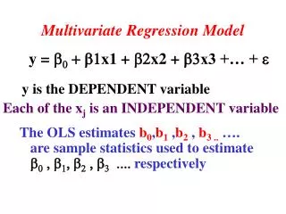
m y = X + e b m n n m ^ y = Xb Multivariate Regression Model: y = Xb + e
The solution of regression problems y = Xb + e When e is minimised: y = Xb Xty = XtXb The “Normal equation”:(XtX)-1Xty = b Minimise with respect to b0, b1,…,bM Condition: XtX must have full rank
Problems • Many x-variables, few objects (measurements) • Correlation between the x-variables det |XtX | 0 (XtX)-1 does not exist! • “Noise” in X
Generalised inverse Generalised inverse:X+ = (XtX)-1Xt Normal equation: b = X+y Biased Regression Methods differ in the way that the Generalised Inverse is calculated
Problem Specification Standards with known concentrations are measured on two highly correlated wavelength. Make a calibration model between the concentrations and the measured intensities at the two wavelengths: c = f(x1,x2)
x2 7 PC1 5 t1 6 t2 x1 3 . 4 . . 1 tN 2 Dimensionality Reduction t, score vector c, concentration vector Quantitative information about the concentration in t
PC1 y ^ ^ y1 t1 = bPC1 t2 y2 . . ^ . . t = f(x1, x2) = f(c) . . tN yN The Regression
^ ^ t1 y1 = bPC1 y - y = bPC1t + e t2 y2 . . ^ . . . . yN tN tt(y - y ) bPC1 = ttt Calculation of the Regression Coefficient
Response (output) variable System y Instrumental (spectral) variables I y = f(X) I X Regression modelling
A X = TPt + E = tapat + E a=1 A y = y+bata + e a=1 Solution 1. Decompose the matrix of spectral data (X) into (orthogonal) latent variables (LVs) 2. Model the dependent variable in terms of the latent-variable score vectors
Scores: t = f (c1, c2, …) Contains quantitative info about the concentrations Loadings: p= f (1, 2, …) Contains qualitative info about the spectra Scores and Loadings
Partial Least Squares (PLS) - best for prediction Principal Component Regression (PCR) - best for outlier checking Regression Methods Combine the methods
= bLV t1 t2 tA y-y orthogonal y = y + bLV1t1 + bLV1t2 + .. + bLVAtA Data described by several Latent Variables Model:
A y - y = bLV,ata + e a=1 A tbt(y - y)= bLV,a tbttLVa + e a=1 zero, except for a=b (y - y)tbt bLV,B= tbt tb Calculation of the regression vector
Latent-Variable Regression Modelling The Modelling process Validation Interpretation (Regr. coeff., loadings) Number oflatent variables (Explained var. in X and Y, Cross Validation, Regr. Coeff., Loadings etc.) OutlierDetection
Cross Validation (statistical validation) i) Divide the samples into a number of groups, ng. ii) For each LV dimension, a=1,2,.., A+1, perform the following calculations:1. Estimate the LV a with group k of samples excluded. 2. Predict the responses for samples in group k. 3. Calculate the squared prediction error for the left-out samples, iii) Repeat step ii)until all samples have been kept out once, and only once, then calculate iv) If SEP(a)<SEP(a-1) go to ii), otherwise stop and select number of dimensions (LVs) in model as a-1, A
Application Example 1 Process industry, where the principal qualities1 of products are linked to chemical composition of raw material and the manufacturing process. 1 O. M. Kvalheim, Chemom. & Intel. Lab. Syst. 19 (1993) iii-iv.
Application Example 2 Environmental sciences, such as the prediction of the diversity of a biological system from instrumental fingerprinting of the chemical environment, principal environmental responses.