Download

1 / 37
370 likes | 544 Views
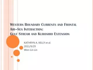
Frontal scale WBC air-sea interaction issues. Some influences. Also. Also Hisashi Nakamura, Shoshiro Minobe, Masami etc. … and the WBC working group…. Outline – summaries and questions. 1. Atmospheric boundary layer response to WBCs, some findings and questions.

E N D
Frontal scale WBC air-sea interaction issues Some influences Also Also Hisashi Nakamura, Shoshiro Minobe, Masami etc … and the WBC working group…
Outline – summaries and questions • 1. Atmospheric boundary layer response to WBCs, some findings and questions. • 2. Deep atmospheric response, some findings and questions. • Importance for mean state • 3. Storm track response to WBCs, some findings and questions. • 4. Feedback onto ocean • 5. Way forward – SST anomalies and climate variability. How to address this – joint model project? Overview slides followed by illustrations– discussion at end?
Response of marine boundary layer to SST gradients • WBCs regions of largest ocean to atmosphere heat flux in midlatitudes (Bunker and Worthington 1976, CLIMODE group, KESS) • Wind and stress correlation with SST over ocean eddies, fronts (reviewed by Xie et al 2004, Chelton et al 2004, Small et al 2008) • Direct stress effects (Liu, also Ralph Foster) – drag coefficient changes across front. Estimates of importance range from ~30% (O’Neill, Small) to 70% (Liu). Stress convergence but no wind convergence a problem for deeper response? • Momentum mixing (Hayes et al 1989) driven by surface instability • Pressure gradients and secondary circulations (Lindzen and Nigam 1987, Small et al 2003, Minobe et al 2008, laplacian of SLP, others). SLP anomalies in KE over warm SST cause cloud formation (winter): in summer warm KE inhibits fog formation (Tokinaga) • Stress proportional to boundary layer height (Samelson) • Refer Spall work, Takatama • Actually mixing (sensible heat fluxes ~ Ts-Ta) important for all mechanisms---- • Precise mechanism not really important – what is important is the magnitude of convergence and/or buoyancy/latent heat flux which may influence troposphere • Climate model requirements: Metrics for atmospheric response: hi-pass SST vs. Usfc.correlation; downwind SST gradient vs. wind stress anomaly (Chelton). Need higher ocean resolution.
Deep response of atmosphere • Liu et al (2007) air temperature anomalies up to 300hPa above Agulhas meanders • Minobe et al (2008) ascent throughout troposphere, upper level divergence and clouds, low level convergence, seasonal modifications • Winter has strong low level convergence, shallow heating – baroclinic instability • Summer has high SSTs, deep heating (weak low level convergence, more latent heating?) Atmosphere preconditioned by fairly unstable thetae profile – warm SST and surface buoyancy leads to deep convection • Also seen in various model experiments (Hand, Kuwano-Yoshida) • Xie, Tokinaga et al (2009/2010/2011??), high level clouds over KE in winter • How large is this effect? Samelson (pers comm) – low level convergence and consequent ascent over GS equivalent to that for a hill of a few hundred meters – is this important? Same question for Agulhas meanders (Liu). • But diabatic heating is large (TRMM, JRA25)
Storm Track Free tropospheric storm track and WBC • Low level baroclinicity important for storm development (Hisashi Nakamura, Hoskins and Hodges ) influenced by ocean front • Hatteras-North Wall temperature gradient - Land-sea contrast modified by WBC? (Cione et al 1993). Upper level vorticity as second independent variable (Jacobs et al 2005). Surface storm track and WBC • Free tropospheric storm track modified by near surface stability • Sampe and Shang-Ping Xie, Terry Joyce, Jimmy Booth work • Ocean baroclinic adjustment (Taguchi, Nonaka, Hisashi) • Ocean front helps fix storm track via sensible heating – restores T • Low level sensible heating counters eddy heat flux Alternative to Hoskins and Valdes idea • Eady growth rate – dependence on stability and horizontal temp gradient (vertical shear) Hisashi – compute growth rate using near surface data • Stability dependent on ocean SST front - Booth • New ‘baroclinicity’ index to replace Cione et al? Decadal variability – SST anomalies in KE potentially influence storm track(Hisashi)
Response to midlatitude SST anomaly • Local linear baroclinic response to diabatic heating (Hoskins and Karoly, Palmer and Sun,) • Feedback from eddy vorticity and heat fluxes may be important, can cause equivalent barotropic response (Peng and Whitaker, Peng et al, Yochanan Kushnir et al 2002) • Time-evolving response shows linear response first (~ a week) followed by effect of eddy fluxes – equilibrium after 2-4 months (Deser et al 2007, JCLI, Frankignoul et al) • Broad, fairly low level heating • How is this changed by narrow, concentrated, possibly deeper heating? • Limited observational evidence for climate response to ocean extratropical SST anomalies (Frankignoul) • Limitations due lack of resolution in Reanalysis- compare with QuikSCAT measurements of surface ‘atmosphere’ and storm track • (local mean response is finescale in atmosphere –minobe- ) • Model experiments need SST anomalies
Response of ocean (1) • Ekman pumping • Stress gradients at the surface due to • SST-wind feedback (Seo et al) and • gradients in surface ocean current (Dewar and Flierl, Small et al – top drag, AMS talk) • Significant effect – O(1) we (Seo), EKE damping of 30% (Small) • Effect of GS currents on fluxes: 10% errors in heat flux, 20% errors in wind stress. How important is this relative to SST effects? (Bigorre) • Also Affects heat flux
Response of ocean (2) • Mode water formation – ’50% at or close to Gulf Stream front ‘ (Joyce, this workshop) • Driven by surface buoyancy fluxes but vertical shear important • High resolution models necessary ?
Schematic from review paper Figure 15. Schematic showing boundary layer response to an ocean frontal boundary. The flow is from cold to warm SST in a situation with (a) strong background winds and (b) weak background winds. Below each panel are horizontal across-front profiles of SST and air temperature Tair. Above is shown the sea surface, with wave height increasing to the right of the SST front. Background winds U at left are incident on the front. A mixed internal boundary layer (gray shading) develops downstream. Circular arrows indicate the presence of turbulent eddies. Forces due to mixing (Fmix, term IV of equation (4a)) and pressure (Fpres, term III) are indicated with thin arrows. Due to these forces the wind profile becomes uniform with height (thick black arrows). To the right are shown vertical profiles of the downstream air temperature anomalies (dashed) and pressure anomalies (solid). Momentum mixing important warm cool Pressure gradient important cool warm Note: upward heat flux (red) from ocean over warm SST warms internal boundary layer Modification to include coriolis effects, thermal wind (O’Neill PhD Thesis)
SST (COL) AND 10M WIND S SST (COL) AND 10M WINDS OBSERVATIONS MODEL HIGH PASS FILTERED SST AND 10M WINDS
LETS LOOK AT MOMENTUM BALANCE TERMS FOR IDEALISED GAUSSIAN EDDIES BACKGROUND WIND Minus Winds accelerate towards low pressure (red) ACCELERATION VECTORS DUE TO GRADP WINDS ACCELERATE TOWARDS LOW PRESSURE Dv/Dt=-GradP/rho+…
Frontal Scale Air-Sea Interaction in High Resolution Versions of the Community Climate System Model • Fully coupled climate simulations with eddy resolving ocean components are technically feasible but still very computationally challenging and costly. • The observed relationships between frontal scale SST structure and low level winds and/or surface stress may provide useful metrics with which to test coupled climate models in this regime that do not require century length integrations. • Local temporal correlation of u10 and sst; Slope of regression of wind stress on sst, div and curl of stress on downwind and crosswind sst gradient; Seasonal cycle of regional differences in these measures • Correlation of high pass sst and low level winds weak with lores ocean model, becomes systematically stronger over frontal regions with hires ocean model. • Coupling between high-pass sst and stress less than ½ observed estimate, independent of model resolution, suggesting intrinsic deficiency of atmos. model PBL physics. 0.5° atm / 1.0° ocn 0.5° atm / 0.1° ocn Correlation High-Pass SST vs. |usrf| 0.5° atm / 1.0° ocn 0.5° atm / 0.1° ocn 0.25° atm / 0.1° ocn Agulhas region stress vs SST regression
Seasonal variation of the updraft response (Kuwano-Yoshida) Figure.B Vertical cross section averaged between 290oE and 310oE for vertical velocity (color,), moisture convergence (thick contours), and saturation equivalent potential temperature (thin contours).
TRMM estimates of diabatic heating North Atlantic North Pacific
Surface sensible heat flux Probability of low-level storm-track axis Anchoring of a storm track by a mid-latitude oceanic frontNakamura, Sampe, Goto, Ohfuchi, Xie (2008 GRL) Oceanic front acts to anchor a storm track and PFJ by restoring near-surface baroclinicity effectively: “oceanic baroclinic adjustment” c.f. conventional baroclinic adjustment due to differential radiative heating (with time scale of 1~2 weeks) c.f., Moisture supply from a warm western boundary current (Hoskins, Valdes 1990)
υ850mb A.B.L. Stability υ10m Predicted and actual surface storm track Results: Atlantic Basin (Jimmy Booth) The surface storm track
Results: Pacific Basin υ850mb A.B.L. Stability υ10m Predicted and actual surface storm track
Storm tracks: That’s the time mean, what about variability?
Confinement of extratropical decadal SST variability into major oceanic frontal zonesNakamura, Kazmin (2003; JGR) importance of oceanic processes atmospheric bridge (basin-scale) DJF climatology of Northward SST gradient (±0.1, 0.3, 0.5, 0.7, …deg./100km) DJF decadal SST variability (COADS) (std. dev. : 0.3, 0.4, 0.5, 0.6 deg.)
100mb SST (Nov) vs Z925 (Jan) –2 mo. 250mb +50m –40m 1000mb 120W 120E 120W 120E Zonal section of height (contoured) and temperature (colored) anomalies for 55N Wintertime basin-scale atmospheric response to quasi-decadal SSTA in the KOE region (Nakamura) Shallow local response and deep, equivalent barotropic response downstream [c.f., Peng et al. (1997)] Feedback forcing by transient eddies along the poleward-shifted storm track on the equivalent barotropic anomalies.
Kushnir et al (2002) – response to low level heating with eddy fluxes included Minobe et al (this workshop)
Narrow heating (Minobe et al 2008) Problems with this: Heating pattern is not an anomaly! Based on annual mean heating (Smooths seasonal changes) No eddy flux feedback Gulf Stream is blocky
Narrow heating (Minobe et al 2008) Deser et al 2007. Fig. 9. (left) Vertically averaged diabatic heating responses for days 2–8 and 45–120 for the (top) SST (right)Vertical profiles of the diabatic heating responses for days 2–8 (thin curve) and days 45–120 (thick curve)
Interannual variability of local forcing from TRMM Analysis is challenging because of patchy nature of rainfall and narrow swath width of PR Perhaps we can start by analysing changes in surface convergence any relationship with SST or rainfall
Eddy Kinetic Energy in Tropical Instability Waves With understress No understress Figure 1. EKE (kgm-1s-2), depth averaged from the surface to 100m. a): Experiment 1. b): Experiment 2. The Ekman pumping anomalies compares well with a rough estimate which assumes that only the understress is modifying the stress. The consequent dissipation has an e-folding timescale of 115 days.
Seasonal variation of the updraft response (Kuwano-Yoshida) Figure.B Vertical cross section averaged between 290oE and 310oE for vertical velocity (color,), moisture convergence (thick contours), and saturation equivalent potential temperature (thin contours). Figure A. Vertical velocity (color, -10-2 Pa s-1) at 200 (left column), 500 (center column) and 850 (right column) hPa for CNTL. (a) (b) (c) Annual mean, (d) (e) (f) in JJA, and (g) (h) (i) DJF. • The updraft extends vertically up to the upper troposphere over the Gulf Stream in summer, while it is restricted the lower troposphere. The vertical thermodynamic profile of troposphere controls the updraft response to the Gulf Stream.