Download
1 / 17
180 likes | 375 Views
Artificial Dissipation. The artificial dissipation term used in FEM is different than in FD,. Note: A is included to match terms in other equations. Artificial Dissipation (cont’d 2). Conservation of Mass:. Conservation of Momentum. Artificial Dissipation (cont’d 3).

E N D
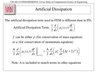
Artificial Dissipation The artificial dissipation term used in FEM is different than in FD, Note: A is included to match terms in other equations
Artificial Dissipation (cont’d 2) Conservation of Mass: Conservation of Momentum
Artificial Dissipation (cont’d 3) Applying method of weighted residuals and integration by parts to the artificial dissipation term in the conservation of mass equation,
New Local System Equations Conservation of mass
New Local System Equations (cont’d 2) Conservation of momentum
Boundary Conditions Implementation of boundary conditions will be done in the same way as for the FD equations.
program hw6c integer nodes(131,2), lnode(2) real kglobal(258,6),klocal(4,4),x(131),svec(258), real area(131),coord(2),phi(2),dphi(2), real larea(2),x(3),w(3),lu(2),lrho(2),lmu(2),mulocal real fvec(258),flocal(4),uvec(131),rhovec(131) real kbound1(2,2),kbound2(2,2)cc initialize variablesc maxnode=131 maxmat=2*(maxnode-2) maxel=130 nlast=10000 dt=1.e-3 dx=0.1 temp=300. gamma=5./3. xi(1)=0.7745966692414830 xi(2)=0.0 xi(3)=-x(1) w(1)=0.5555555555555560 w(2)=0.8888888888888890 w(3)=w(1) Declare variables and Initialize certain variables
do 10 i=1,maxnode c x(i)=(i-1)*dx c if(x(i).le.3.0)then c area(i)=4-2./3.*x(i) c else c area(i)=0.6*(x(i)-3.)+2. c endif c 10 continue c do 20 i=1,maxel c nodes(i,1)=i nodes(i,2)=i+1 c 20 continue Set up nodal coordinates, the area at each node, and the connectivity between local and global node numbers
do 500 it=1,nlast c do 40 j=1,6 c do 30 i=1,maxmat c kglobal(i,j)=0.0 c 30 continue c 40 continue c do 200 ie=1,maxel c lnode(1)=nodes(ie,1) lnode(2)=nodes(ie,2) lrho(1)=rhovec(nodes(ie,1)) lrho(2)=rhovec(nodes(ie,2)) lu(1)=uvec(nodes(ie,1)) lu(2)=uvec(nodes(ie,2)) coord(1)=x(nodes(ie,1)) coord(2)=x(nodes(ie,2)) larea(1)=area(nodes(ie,1)) larea(2)=area(nodes(ie,2)) lmu(1)=0.125*lrho(1)*abs(lu(1))*dx lmu(2)=0.125*lrho(2)*abs(lu(2))*dx hlocal=coord(2)-coord(1) hlocalinv=1./hlocal Initialize sparse matrix. Loop through all the elements, one at a time. Set up local system variables at the two local nodes for the element of interest
do 110 j=1,2 c do 100 i=1,2 c iloc=2*i-1 jloc=2*j-1 c do 60 jinit=1,4 c do 50 iinit=1,4 c klocal(iinit,jinit)=0.0 c 50 continue c 60 continue c do 80 nint=1,3 c xlocal=0.5*(xi(nint)*hlocal+(coord(2)+coord(1))) phi(1)=hlocalinv*(coord(2)-xlocal) phi(2)=hlocalinv*(xlocal-coord(1)) dphi(1)=-hlocalinv dphi(2)=hlocalinv alocal=larea(1)*phi(1)+larea(2)*phi(2) dalocal=larea(1)*dphi(1)+larea(2)*dphi(2) ulocal=lu(1)*phi(1)+lu(2)*phi(2) rholocal=lrho(1)*phi(1)+lrho(2)*phi(2) mulocal=lmu(1)*phi(1)+lmu(2)*phi(2) Loop through i,j, and also Set up indices of p,q. Zero out local matrix Apply 3 pt Gauss quadrature.
c k_ij^(11) c term=2.*alocal/dt*phi(i)*phi(j)-ulocal* ! alocal*dphi(i)*phi(j)+0.5*mulocal*(alocal* ! dphi(i)+phi(i)*dalocal)*dphi(j) klocal(iloc,jloc)=klocal(iloc,jloc)+term* ! w(nint)*hlocal/2. c c k_ij^(12) c term=-rholocal*alocal*dphi(i)*phi(j) klocal(iloc,jloc+1)=klocal(iloc,jloc+1)+ ! term*w(nint)*hlocal/2. c c k_ij^(21) c term=alocal/dt*ulocal*phi(i)*phi(j)-0.5* ! ulocal**2*alocal*dphi(i)*phi(j)-temp/(2* ! gamma)*(alocal*dphi(i)+phi(i)* ! dalocal)*phi(j) klocal(iloc+1,jloc)=klocal(iloc+1,jloc)+ ! term*w(nint)*hlocal/2.
c k_ij^(22) c term=alocal/dt*rholocal*phi(i)*phi(j)- ! rholocal*ulocal*alocal*dphi(i)*phi(j)+0.5* ! mulocal*(alocal*dphi(i)+phi(i)*dalocal)*dphi(j) klocal(iloc+1,jloc+1)=klocal(iloc+1,jloc+1)+ ! term*w(nint)*hlocal/2. c c f_i^(1) c term=2.*rholocal*ulocal*alocal*dphi(i)-mulocal* ! rholocal*(alocal*dphi(i)+phi(i)*dalocal) flocal(iloc)=flocal(iloc)+term*w(nint)*hlocal/2. c c f_i^(2) c term=rholocal*ulocal**2*alocal*dphi(i)+ ! (temp/gamma*rholocal-mulocal*ulocal)* ! (alocal*dphi(i)+phi(i)*dalocal) flocal(iloc+1)=flocal(iloc+1)+term* ! w(nint)*hlocal/2. c 80 continue c 100 continue c 110 continue
idfree=(lnode(1)-2)*2 c if(ie.eq.1)then c do 130 jj=1,2 c do 120 ii=1,2 c kglobal(idfree+2+ii,jj+2)=kglobal(idfree+ii,jj+2) ! +klocal(ii+2,jj+2) kbound1(ii,jj)=klocal(ii+2,jj) c 120 continue c 130 continue c else if(ie.eq.maxel)then c do 150 jj=1,2 c do 140 ii=1,2 c kglobal(idfree+ii,2+jj+2)=kglobal(idfree+ii,2+jj+2)+ ! klocal(ii,jj+2) kbound2(ii,jj)=klocal(ii,jj+2) c 140 continue 150 continue
else c do 180 jj=1,4 c do 170 ii=1,2 c kglobal(idfree+ii,2+jj)=kglobal(idfree+ii,2+jj)+klocal(ii,jj) kglobal(idfree+2+ii,jj)=kglobal(idfree+ii,2+jj)+klocal(ii+2,jj) c 170 continue c 180 continue c endif c 200 continue c c Boundary Conditions c c Solution of Matrix c If not in first or last element, transfer entire local matrix to global matrix. Boundary condition and matrix solution left for your project
c resetting the values for the next iteration c do 250 i=1,maxnode-2 c i1=i*2-1 rhovec(i+1)=svec(i1)+rhovec(i+1) uvec(i+1)=svec(i1+1)+uvec(i+1) c 250 continue c uvec(1)=2.*uvec(2)-uvec(3) uvec(maxnode)=2.*uvec(maxnode-1)-uvec(maxnode-2) rhovec(1)= rhovec(maxnode)=2*rhovec(maxnod-1)-rhovec(maxnode-2) c 500 continue c stop end Note: index shift to account for reduction ff 1st and last set of rows of matrix equation Solution at first and last node is given, but may not be necessary.