Download
1 / 40
420 likes | 645 Views
Artificial dissipation methods for Euler equations V. Selmin. Multidisciplinary Computation and Numerical Simulation. Euler equations properties. Conservation law form: Unknowns & Flux vector: State equation: Non conservative form:. Euler equations. Euler equations properties.

E N D
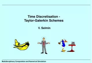
Artificial dissipation methods for Euler equations V. Selmin Multidisciplinary Computation and Numerical Simulation
Euler equations properties Conservation law form: Unknowns & Flux vector: State equation: Non conservative form: Euler equations
Euler equations properties Hyperbolicity: Let be a linear combination of the fluxes where is a nonzero vector. The system is hyperbolic if the the Jacobian matrix has only real eigenvalues. Eigenvector and eigenvalues: The eigenvectors form the matrix that diagonalises : Jacobian matrix decomposition: The following decompositions is also introduced: The matrices and are diagonalised by the transformation : Flux homogeneity Euler fluxes are homogeneous of degree one with respect to W Euler equations
Finite Volume/Finite Element Node-Centred finite volume Discretisation of the integral equation: Discrete equation: Consistency: Conservative systems: Second-order spatial approximation: Finite Volume/Finite Element Formulation
Finite Volume/Finite Element Positivity Scalar equation: Discrete equation: Condition on scheme positivity: Monotone numerical scheme: Extension to systems of equations: Finite Volume/Finite Element Formulation
Entropy Condition The weak solutions are not univocally defined for the partial differential problem: different solutions may satisfy the initial condition. An additional principle is then needed for the settlement of a solution physically acceptable. Let consider the hyperbolic equation where f(u) is a nonlinear function of the uknown. The eligible solution is the limit when of the solution of the viscous problem: Oleinik has shown that the eligible solution must satisfy the following inequalities for . These relations are called entropy condition. Entropy condition
Flux Difference Splitting A central role is played in the algorithm by the modelling of the interactions of fluxes at the interfaces of adjacent grid cells. Two distinct sets of state quantities must be combined into one single set of numerical fluxes at the interface. In the following, some upwind related tecnologies which may be used to build the numerical flux will be discussed. Flux Difference Splitting: Let consider the Riemann problem governed by the one-dimensional inviscid flow equation: Roe’s scheme may be interpreted as an approximate Riemann solver based on the linearised equation: The matrix has to satisfies the following properties: 1- (Consistency) 2- has a complete set of real eigenvalues and eigenvectors (Hyperbolicity) 3- (Conservation propertty) 4- When the two states are connected through one discontinuity, the discontinuity can be reproduced exactly. Conditions 1 and 3 have to be satisfied when the Jacobian is computed at an average state: Flux Difference & Vector splittings
Flux Difference Splitting Roe introduced the following average operator for a polytropic ideal gas: The average operator is in general valid for a gas whose pressure law allows the flux F to be an homogeneous function of degree one in the conservative variables. As the pressure is expressed in the general form that means the following condition has to be satisfied: The numerical flux on this approximate Riemann solver may be expressed by Another approximate Riemann solver , with similar properties, is due to Osher: Numerical flux not differentiable Crisp representation of discontinuities Does not satisfy the entropy condition Allows expansion shocks Numerical flux differentiable Integration path // to the eigenvectors of A Satisfy the entropy condition Flux Difference & Vector splittings
Flux Vector Splitting In the case of Flux Vector Splitting (FVS), the numerical flux across an interface separating two states and is considered as the sum of two parts and that should possess the following desirable properties: 1- (consistency to the governing equations), 2- must have all the eigenvalues , must have all the eigenvalues 3- must be continuous with for , for where M is the Mach number normal to the interface 4- The components of and together must reproduce the symmetry of F with respect to M (all other quantities held constant), that is if 5- must be continuous Restriction (3) ensures that in supersonic regions leads to standard upwind differencing. In general, the flux decomposition is chosen in such a way that are homogeneous of degree one. The numerical flux may be expressed as which can be rewritten to make it to look like the Osher’s formula The integration is independent of the path since is a perfect gradient Flux Difference & Vector splittings
Enlargement of the grid Mach number contours Symmetry axis+body nodes Computational domain (65x41) nodes Test case: hypersonic flow around a cylinder The test case corresponds to compute a flow around a cylinder section. In this case, a detached choc of high intensity (from M=8 to M=0.3929) is present in front of the body. The flow, being subsonic behind the shock, becomes supersonic at approximatively 29% of the cylinder radius. Flux Difference & Vector splittings
Expansion discontinuity “Carbuncle” effect in Roe scheme Roe’s scheme & the entropy condition As already anticipated previously, the numerical flux of the Roe scheme may be written for multidimensional problems according to where the quantities in the dissipation term are computed by using the average proposed by Roe and To have a zero value of the eigenvalues independently of the difference may lead to a violation of entropy condition, whereas the dissipation matrix may become singular when . Flux Difference & Vector splittings
Entropy condition not satisfied Entropy condition satisfied Roe’s scheme & the entropy condition Harten proposed to regularize the dissipation matrix by using the following correction of the eigenvalues: Flux Difference & Vector splittings
Multidimensional extension A method to extend the upwind schemes to multidimensional problems is based on the property of the Euler’sequations to be invariant with respect to a rotation of the coordinate axis. Let be a linear combination of the fluxes where is a nonzero vector of real quantities. A local rotation of the velocity vector is defined in the following way: The state is transformed into the state Moreover, applying the the rotation to the flux allows to describe the flux vector in a one dimensional fashion Finally, the inverse transformation express the different flux in the original frame The eigenvalues of the Jacobian matrix are not modified Flux Difference & Vector splittings
Matrix Dissipation Operator The matrix dissipation flux may be described in a straightforward way for the Euler equations. In the rotated frame, the matrix dissipation operator takes the form where It may be demonstrated that by using Roe’s averages and , we obtain Matrix Dissipation Operator
Matrix Dissipation Operator The matrix dissipation flux becomes The coefficients are functions of the eigenvalues of the system and take the form: which may be expressed with respect to the Mach number normal to the interface according to Matrix Dissipation Operator
Matrix Dissipation Operator • The first term of the matrix dissipation operator is able alone to maintain the monotonicityof Roe scheme • The second term is a diffusive operator acting only in subsonic regime. • The third term is an antidiffusive operator that acts both in subsonic and supersonic regime. Matrix Dissipation Operator
Matrix Dissipation Operator Matrix Dissipation Operator
Matrix Dissipation Operator In order to enforce the entropy condition, the coefficients may be regularised according to Matrix Dissipation Operator
Isoenergenetic flows A desirable property of a numerical scheme for the solution of the Euler equations is its capability to reproduce an isoenergenetic steady state flow. Whether the discretisation of the convective flux might provide a solution which satisfies the solution, this no more true when the dissipation operator is added to the numerical scheme. To obtain a scheme which satisfies this property, the following dissipative flux is introduced Properties: 1- The flux preserves the monoticity of the numerical flux. 2- Essential property in order to obtain accurate stagnation temperature 3- Enthalpy damping techniques may be used to speed up convergence of transonic flows solution. Total enthalpy constant over the entire field Matrix Dissipation Operator
Isoenergenetic flows A more compact expression of may be obtained by rewritting the scheme with respect to the coefficients and only. Characteristic variables: may be expressed according to Matrix Dissipation Operator
Scalar Dissipation In the context of centered approximations, a simpler approximation for the dissipation operator may be obtained by replacing in the matrix dissipation operator all the eigenvalues of the Jacobian by its spectral radius: The modification leads to the following scalar dissipation operator which preserves the monoticity of the scheme,but it is more dissipative. In the original frame, the scalar dissipation operator may be transformed according to: Scalar Dissipation Operator
Van Leer Flux Vector Splitting A very promising study for splitting the flux has been introduced by Van Leer. He deduced formulas that satisfy the basic requirements , but with the following additional properties: 1- must have one eigenvalue vanishing for . 2- , like , must be polynomials in M and of the lowest degree. Constraint (1), that van Leer considered crucial, makes it possible to build numerical shock structures using two interior zones. The requirement (2) makes the splitting unique. The formulas for are given in terms of the Mach number. For supersonic and sonic flows, , we have and for subsonic flow, , Split fluxes continuously differentiable Valid only for a perfect gas Flux Vector Splitting
Montagné Flux Vector Splitting A more physical way to build a flux splitting consists in approaching the conservative laws by a collisionless Boltzmann equation. Each state is split into group of particles which are distributed according to their velocities. The density law of particles, which obeys a Maxwell distribution in the kinetic theory of gases, must be approximated by a simpler distribution law. The fluxes and are defined by considering the particles with positive and negative velocities, respectively. In addition, it is requested that reduces to F for supersonic flows with a positive (negative) velocity. The formulas for are given in terms of the Mach number. For supersonic and sonic flows, , we have and for subsonic flow, , Split fluxes not always continuously differentiable Valid not only for a perfect gas Property (1) not satisfied Flux Vector Splitting
Enthalpy preserving Flux Vector Splitting The new splitting is based on the following heuristic consideration: 1- The fluxes of van Leer scheme are continuously differentiable and are expressed in a general form (OK). 2- The fluxes of the Boltzmann type scheme are constinuously differentiable and are very close to the corresponding fluxes of the van Leer type (OK). 3- For the components of the third fluxes, any of the the previous schemes can be retained. In addition, they do not satisfy the condition of constant total enthalpy for isoenergenetic steady flows. They can be repaired by taking . Moreover, if fluxes are continuously differentiable, it will also the case for . For supersonic and sonic flows, , we have and for subsonic flow, , Split fluxes continuously differentiable Valid for any gas Very simple expressions Flux Vector Splitting
Multidimensional extension Applying the rotation to the flux allows to split the flux in a one-dimensional fashion: After splitting , the inverse transformation gives the following relations for the flux splitting: Then the numerical flux reads For multidimensional applications, the proposed flux splitting is described by the following formulas. Indicating by the quantity , for , we have and for subsonic flow, Flux Vector Splitting
j+ j i+2 i i+1 i- i i-1 Extension to second order spatial accuracy All upwind schemes (FDS, FVS) may be interpreted as built from a centred discretisation (second-order accurate) spatial approximation + an artificial dissipation term (first-order accuracy) The schemes are first-order accurate in space. In general, artificial dissipation is needed only at discontinuities, thus development of sensors that identify discontinuities (or rapid change of the solution) and monitor the level of dissipation by using the sensor. The quantities and are replaced by the following expressions where s and are parameters, and are “extrapolated” values of the unknowns. N.B.: The values of and may be used in the evaluation of all the terms of the FDS or FVS schemes or only for the evaluation of the dissipative term. FDS FVS Second order accuracy
Extension to second order spatial accuracy The variation may be expressed according to Thus, Then, in order to avoid oscillations in the numerical solution, in particular near shocks, the extrapolation has to be limited by varying the switching factor s , which is controlled by the solution itself. Typical formulation of such limiters are given by where is a small number ( ) preventing division by zero in regions of null gradients. These limiter formulations react to the local gradient and to the curvature of the solution, i.e. Thus, in regions of weak changes of W , the limiter remains nearly to one, but for strong changes the value decreases and the scheme reduces the accuracy generating a stronger numerical simulation. First-order scheme Higher-order scheme Second order accuracy
j+ j ej i ei i- j* i* Extension to second order spatial accuracy Methods to computed extrapolated variables 1- Centred gradient: This formulation works well for subsonic and transonic flows, but not for high supersonic flows, for which it is not able to forecast the correct slope of the solution upstream or downstream of the nodes i and j, respectively, since the gradient approximation is centered. 2- Upstream/downstream element gradient: This formulation works well for subsonic, transonic flows and supersonic flows. It forecasts the correct slope of the solution upstream or downstream of the node i and j, respectively. Nevertheless, it needs additional data structures for the computation of the gradient on the element. 3- Upstream/downstream segment variation: This formulation works well for subsonic, transonic flows and supersonic flows. It forecasts an approximation of slope of the solution upstream or downstream of the node i and j, respectively. It gives a good information for the computation of the limiter s, but the approximation for the third-order operator is less accurate. It needs very few additional data structure information to work. The nodes i* and j* are selected in such a way that the segments i-i* and j-j* minimise the scalar product with the segment i-j Second order accuracy
Extension to second order spatial accuracy • Alternative methods to compute the third-order term • where • Remarks: • 1- The use of the operator leads to a final discretisation similar to those of a directional fourth-order derivate • 2- The use of the operator leads to a final discretisation similar to those of a biharmonic operator • 3- The use of the harmonic operator leads to a more robust discretisation for multidimensional grids with deformed • elements. Second order accuracy
Extension to second order spatial accuracy Special treatments for the scalar dissipation In the classical scalar artificial method, it is preferred to use the following expression for the variation: with where the discontinuity sensors are expressed in terms of pressure variations Remarks: 1- The aim of the background dissipation is to improve the ability of the scheme to damp high frequency modes in smooth part of the flow. 2- are adjustable parameters. 3- The value of is limited to 1 because we know that with this value the scheme maintains monoticity. 4- The term is substract from to cut off the fourth order difference operator, which could otherwise cause an oscillation in the neighbourhood of a shock wave. shock capturing background dissipation Second order accuracy
Modelling of High Speed flows At hypersonic speed, a strong shock appears in front of an aerospace vehicle. The compression of the gas through the shock is associated with an increase in temperature. Through the shock wave , the total enthalpy is constant and along a streamline, we can write If the velocity is very large, . A strong shock causes a large variation of the fluid velocity. Thus, in front of the vehicle, . Consequently, we have This means that almost all the kinetic energy is transformed into heat, resulting in a very high temperature in the region between the body and the shock. An important characteristic of hypersonic phenomena is then the transformation of an hypervelocity flow into an hyperenthalpy one. Another characteristic is that a part of that energy is transformed into chemical energy, as a consequence of (i) excitation of the internal degree of freedom of molecules, (ii) dissociation of molecules, (iii) ionisation. These phenomena are endothermic and the final temperatures reached are much lower than those obtained for a non-reactive gas. Moreover, in these conditions, the properties of air are modified. The chemical composition of air can be approximately subdivided into the following regimes: 1- T<2500K. The chemical composition is substantially that at room temperature. 2- 2500<T<4000K. The oxygen dissociation regime, no significant nitrogen dissociation,slight nitric oxyde formation 3- 4000<T<8000K. The nitrogen dissociation regime, oxygen fully dissociated. 4- t>8000K. Inonization of the atomic constituents. h: specific enthalpy Modelling of high speed flows
T = temperature = energy of formation = mass fraction = specific heat at constant volume = energy of vibration = universal gas constant = molar mass Modelling of High Speed flows The model of a real gas can be described as a mixture of perfect gases which are subject to chemical reactions. The state law must take into account , on one hand, the species decomposition and, in another hand, the exitation of internal degrees of freedom of atoms and molecules (translation, rotation, vibration). The internal energy takes the form Note that Using Dalton’s law, the pressure is given by The specific enthalpy is written according to Modelling of high speed flows
Modelling of High Speed flows The following alternatives for the definition of the ratio of specific heats may be introduced: 1- True ratio of specific heats 2- Equivalent relating pressure to internal energy and density 3- Equivalent relating sound speed to pressure and density 4- Ratio of specific heats of the frozen flow Modelling of high speed flows
Non-reactive flows A gas formed by standard air (oxygen+nitrogen) is assumed and the vibrational degrees of freedom of the diatomic molecules are neglected. We obtain a perfect gas with constant ratio of specific heats, i.e. The pressure and the sound speed can be expressed in a simple way as a function of the conservative variables: Remarks: 1- The upwind schemes described previously have been build in such a way they satify the condition of total enthalpy at steady state. That is true for first-order scheme. But, special care must be taken when employing the second order one. The standard procedure is to adopt the primitive variables as sensor for the limiters, which does not satisfy the property. The total enthapy per unit volume has to be used instead of pressure. 2- The upwind formulas depends of five quantities . The limiting procedure is performed on only three of them. This is possible because a constant specific heats ratio is assumed. 3- For hypersonic flows, a drawback is the use of the static speed of sound that control the eigenvalues. In strong expansions, this quantity becomes very small. In this case, it is suggested to use the critical sound speed instead: which does not influence the total flux F and approaches the static speed of sound at the sonic points. 4- The critical sound speed is proportional to the square root of the total enthlapy and is therefore constant for isoenergenetic Euler flows. That leads to a gain in robustness of the solver Modelling of high speed flows
Reactive flows The laws governing chemical reactions have been coupled with the Euler solver. At each iteration of the time integrator, the Euler code provides and update for . The mass fractions are computed by solving a set of nonlinear algebaric equations in the case of chemical equilibrium and a set of partial differencial equations in the case of chemical non-equilibrium. The temperature is computed by expressing the identity of the internal specific energy written in terms of “fluid motion quantities” and “chemical ones”: The outcome is used to update the other thermodynamic quantities in preparation of the next step. The desirable properties that a FVS schemes should possess are: 1- (consistency to the governing equations) 2- must be continuous, with 3- must have all eigenvalues must have all eigenvalues Remarks 1- In the definition of the upwind we have a switch at . The efficiency of the scheme depends on the definition given to the sound speed. Property ( 1) is always satisfied independently of the definition of the sound speed. To ensure that in supersonic regions property (2) is satisfied, we might use the sound speed as it appears in the true eigenvalues of the system: Modelling of high speed flows
Reactive flows 2- Some authors prefer to employ a “false sound speed” approach based solely on satisfaction of property (1): whose value is closer to that obtained from available experimental data. 3- Other choices for the definition of the sound speed are a priori possible. However property (3) has to be satisfied. The consequence is that and can not vary independently. In particular, it can be shown that must be greater or equal to . 4- Contrary to non-reactive flows, the specific heats ratios for reactive flows are no longer constant. Then, it is propose to perform the limiting procedure also to and for second-order accurate computations. 5- The concept of critical sound speed has been extended to reactive flows according to Modelling of high speed flows
Iso-Cp contours Computational domain (65x41) nodes Iso-Pt contours Non reactive flows around a blunt body A first test of the numerical scheme has been made for a flow around a half cylinder at . The freestream conditions are taken to approximatively correspond to the standard atmosphere at the altitude of 75 km ( ). 1- scheme a: first-order scheme 2- scheme b: second-order scheme with limitation on 3- scheme c: second-order scheme with limitation on Modelling of high speed flows
Entropy generation along stagnation streamline Total enthalpy residual versus iterations Stagnation temperature versus iterations Non reactive flows around a blunt body Better accuracy of the second order schemes (b & c). Sheme c allows better accordance with respect to entropy generation and stagnation temperatures levels Modelling of high speed flows
Non reactive flow Reactive flow Iso-Cp contours Non reactive flow Reactive flow Iso-Temperature contours Reactive flows around a blunt body The results obtained on the previous case are illustrated now with the hypothesis of reactive flow in thermodynamic equilibrium. Comparisons with non-reactive flow results show that the shock has considerably moved towards the body. The temperature level is considerably reduced and the stagnation temperature is now approximatively 22% of the corresponding non-reactive flow stagnation temperature. Diatomic Oxygen Diatomic Nitrogen Mass fractions for Oxygen and Nitrogen Modelling of high speed flows
Summary 1- Augmented dissipation schemes have been developed for generalised finite volume schemes. 2- Flux Difference Splitting and Flux Vector Splitting schemes may be re-interpreted as a central scheme with augmented dissipation operator, but are first-order accurate schemes 3- Augmented dissipation has to be activated where discontinuities are present, but has to vanish in regions where the solution is regular 4- Numerical schemes have been developed in such a way that total enthalpy is constant for iso-energenetic steady flows (needed in order to obtain accurate stagnation temperature value) In particular, the variables on which limitation is performed have to be accurately chosen. 5- The treatment of high enthalpy non-reactive and reactive flows has been discussed. →extension to finite elements schemes is automatic →introduction of limiters and shock sensors Modelling of high speed flows