Measurements of Upper-Ocean Turbulence and Air-Sea Interaction during VOCALS- REx

1. Measurements of Upper-Ocean Turbulence and Air-Sea Interaction during VOCALS-REx Chris Zappa (LDEO) Tom Farrar (WHOI) Deborah LeBel (LDEO) Leah Trafford (WHOI) Robert Weller (WHOI)

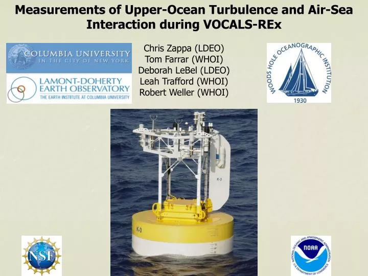
2. Measurements of Upper-Ocean Turbulence and Air-Sea Interaction during VOCALS-REx Outline: Introduction: Conventional turbulence measurements in the open ocean Turbulence measurements with an Pulse-Coherent Doppler Sonar on a surface mooring: Why use an PCDS? Approach Processing and measurement noise Results: 9-months of turbulent dissipation at an open-ocean site Results: Scaling with MO Similarity Theory Results: Periodicity in Dissipation

3. Conventional Approach to Open-Ocean Turbulence Measurements • Free-fall microstructure profilers deployed from ships (e.g., Oakey, 1982; Moum et al., 1995; Gregg, 1998) • Typical sensor package: • CTD • 2 fast-response micro-temperature probes • 2 micro-shear probes • These ship-based measurements are expensive. (Ships cost >$20k/day and the measurements require ~3 people working around the clock.) • Typical data sets are 2 weeks long.

4. Typical 11-Day Data Set (Lombardo and Gregg, 1989) Surface heat flux (units of 100 W/m2) Nighttime cooling Solar heating 10 m Turbulent kinetic energy dissipation 30 m 50 m 70 m

5. Turbulence is Patchy and Episodic Two dissipation estimates from casts 7 minutes apart (from Shay and Gregg, 1986): -20 m -40 m -60 m Dissipation varies by a factor of ~100 between the two casts, for no obvious reason other than the intermittency of turbulence We need a way of making sustained, time-series measurements!

6. Turbulence Measurements from a Surface Mooring • We need sustained time-series measurements of turbulence properties (like turbulent dissipation). • To understand those measurements, we also need time series of: • Surface forcing (e.g., heat flux, wind stress) • Surface waves • Evolution of non-turbulent temperature, salinity, and velocity • Ideally, we’d like all of these measurements sampled at once/hour for many months.

7. Turbulence Measurements from a Surface Mooring • We need sustained time-series measurements of turbulence properties (like turbulent dissipation). • To understand those measurements, we also need time series of: • Surface forcing (e.g., heat flux, wind stress) • Surface waves • Evolution of non-turbulent temperature, salinity, and velocity • Ideally, we’d like all of these measurements sampled at once/hour for many months. • There is really only one way to do all of this: use a surface mooring, with a buoy anchored to the sea floor. • People have been pursuing this for some time using conventional microstructure-profiler techniques (e.g., Lueck et al., 1997; Moum and Nash, 2009). • There are some serious difficulties related to mooring motion.

8. Pulse-Coherent Doppler Sonar for Turbulent Dissipation on a Surface Mooring • Advantages: • Spatial fluctuations of velocity can be estimated without using the frozen-field approximation. • A sample can take only ~1 ms to collect. This helps avoid errors due to platform motion. • Things to worry about: • The turbulent wake of the mooring. • The time taken to make a profile estimate needs to be as short as possible to avoid “smearing” the small-scale turbulence. • (For example, if pings are averaged over ¼ sec and mean flow is 40 cm/s, the minimum resolved length scale is 10 cm.) • The turbulent velocity fluctuations in the open ocean are very weak • (< 1 cm/s) • (4) There is a tradeoff between length of profile (i.e., range) and the maximum velocity that can be unambiguously measured. • (This is because the instrument actually measures a phase shift between returned signals.)

9. VOCALS-REx: “VAMOS Ocean-Cloud-Atmosphere-Land Study Regional Experiment” Primary oceanographic goal: Understanding why SST is cool in the Southeast Pacific October 2008 mean Sea Surface Temperature NSF funded us to instrument 6 depths with Aquadopp HR-Profilers to study mixed-layer turbulence in the VOCALS experiment °C Air-sea flux mooring since 2001 (Bob Weller, WHOI) SST data: AMSRE satellite microwave, courtesy of Remote Sensing Systems

10. Pulse-Coherent Doppler Sonar for Turbulent Dissipation on a Surface Mooring A single horizontal beam measures a ~1.5-m profile with ~3-cm resolution, which can be used for inertial-subrange estimates of dissipation (i.e., fitting a -5/3 power law to velocity spectra) As we configured them, the instruments made a single velocity profile estimate in about 2 ms and averaged 20 of these estimates into ¼ second ensembles. With the extended housing and extra data logger, the instruments collected about 540 profiles at 4 Hz, every hour for one year.

11. Pulse-Coherent Doppler Sonar for Turbulent Dissipation on a Surface Mooring We deployed these instruments at 6 depths in the upper 100 m. 5 out of 6 instrument pairs came back looking like this. We did get good data from an instrument pair at 8.4-m depth (above the spot where the mooring broke).

12. Theoretical Measurement Noise as a Function of Measured Ping-to-Ping Correlation (Theoretical expression from Zedel et al., 1996) Measurement noise (mean square) = ping-to-ping correlation = sound wavelength (~1 mm) = ping time separation Predicted noise, divided by . (20 ping pairs per ensemble)

13. Theoretical Measurement Noise as a Function of Measured Ping-to-Ping Correlation (Theoretical expression from Zedel et al., 1996) Measurement noise (mean square) = ping-to-ping correlation = sound wavelength (~1 mm) = ping time separation 9 months of data (1.8M profiles)  This theoretical expression really works!

14. Estimating Dissipation using an “Inertial Subrange” Fit = wavenumber (i.e., 2π/wavelength) A = constant, ~ 0.557 = turbulent dissipation = velocity spectrum Wavenumber range chosen for fit– noise is an issue here

15. Theoretical Noise to Make Choices in Processing (Theoretical expression from Zedel et al., 1996) Measurement noise (mean square) Predicted noise, divided by . (20 ping pairs per ensemble)

16. Theoretical Noise to Make Choices in Processing (Theoretical expression from Zedel et al., 1996) Measurement noise (mean square) Given ϵ, we expect a certain turbulent velocity

17. Theoretical Noise to Make Choices in Processing (Theoretical expression from Zedel et al., 1996) Measurement noise (mean square) Given ϵ, we expect a certain turbulent velocity Target ϵ

18. Theoretical Noise to Make Choices in Processing (Theoretical expression from Zedel et al., 1996) Measurement noise (mean square) Given ϵ, we expect a certain turbulent velocity By averaging 5 velocity bins and excluding R2<60, the noise should be low enough Target ϵ

19. The Result: 9-Month Time Series of Dissipation (Is it correct?)

20. The Result: 9-Month Time Series of Dissipation (Is it correct?)  We can scale this against “Monin-Obukhov similarity theory”, which says that ϵ should scale with wind stress, surface heat flux and depth.

21. Monin-Obukhov Similarity Theory Scaling  We can scale this against “Monin-Obukhov similarity theory”, which says that ϵ should scale with wind stress, surface heat flux and depth.  Turbulent Dissipation Rate Stress Scaling  Turbulent Dissipation Rate Buoyancy Scaling

22. The Result: 9-Month Time Series of Dissipation (It is looking pretty good.)

23. The Result: 9-Month Time Series of Dissipation (It is looking pretty good.)

24. Monin-Obukhov Similarity Theory Scaling 9 months of data (8.4 m), destabilizing surface buoyancy flux MO stress scaling should hold for z/-L<<1

25. Monin-Obukhov Similarity Theory Scaling: Kansas 9 months of data (8.4 m), destabilizing surface buoyancy flux MO stress scaling should hold for z/-L<<1 “Universal” vertical structure function from Kansas mast experiment

26. Monin-Obukhov Similarity Theory Scaling 9 months of data (8.4 m), destabilizing surface buoyancy flux MO buoyancy scaling should hold for z/-L>>10

27. Periodicity in Dissipation Diurnal Inertial

28. Periodicity in Dissipation • We find a near inertial signal in the turbulent dissipation • We are actively working to understand where that comes from. • It would be nice to have other depths, but we lost them. • We don’t find a strong inertial signal in the wind stress scale, ετ • Is the shear at the base of the mixed layer coherent with surface dissipation at the inertial period? • Check PWP to see if there is an inertial signal in the dissipation • Consistent with the VOCALS hypothesis. • The entrainment of cool fresh intermediate water from below the surface layer during mixing associated with energetic mixed-layer near-inertial oscillations is an important process to maintain heat and salt balance of the ocean surface layer in the SEP.

30. With high resolution velocity data and fluxes calculated, we are in an excellent position to examine the dominant mechanisms of turbulent production. Following boundary layer similarity scalings, the calculated dissipation is scaled by ετ (wind stress dominance) and by the buoyancy flux (buoyancy dominance). All profiles with z/-L, where L is the Monin-Obukov length, are shown above. z/-L = 1 corresponds to a depth where the wind stress and the buoyancy flux contribute equally to the production of turbulence; z/-L > 1 would correspond to a buoyancy-dominated regime, and z/-L < 1 to a wind-stress dominated regime. It is clear that z/-L = 0.1 grossly marks the transition betwen buoyancy-scaling and stress-scaling adequate representing the dissipation levels.

31. Lombardo and Gregg (1989) presented a similar analysis of profiles taken over 11 days at 34N, 127W. Applying the same boundary layer similarity scalings, they found that stress dominated when z/-L < 1 and buoyancy when z/-L > 10. We note that unlike their results, our scaled dissipation does not approach an asymptote of 1. Their results used a depth-averaged ratio, while we present here a point measurement at 10 m depth; their results incorporated a great deal more data with lower dissipations farther down in the water column. We also point out that our transition between the two regimes is closer to z/-L < 0.1. A comparison of day and night profiles indicates that all the strongly stress-dominated profiles occur during the day. In fact, it appears that wind stress-generated turbulence is limited to the daylight hours, while buoyancy generation dominates at night. During the daytime, z/-L < 1 for all but a few profiles, and all of the buoyancy-scaled dissipation ratios indicate an upward trend with decreasing values of z/-L; as L becomes deeper, the buoyancy scaling does an increasingly poor job of representing the observed dissipation. Below z/-L, the stress-scaled ratio shows no such trend. The night profiles, however, show that all of the stress-scaled data follow an increasing trend as z/-L becomes increasing larger; as L shallows, the stress scaling does an increasing poor job of predicting the dissipation values.

32. 13 Seconds of Data: Stepping through Quality Control

33. 13 Seconds of Data: Measured Correlation Key Parameter

34. 13 Seconds of Data : Low Correlations Excluded, Data Unwrapped

35. 13 Seconds of Data : After Initial Quality Control

36. A long time series of upper-ocean turbulent dissipation from a deep-ocean surface mooring equipped with Nortek HR Profilers Conclusion: • Aquadopp HR-Profilers appear capable of providing reasonably low-noise dissipation estimates on a moving platform, over a long time period. • This will probably become increasingly true as more people use them. • I had to discard about 97% of the data to reach this low noise level. • The theoretical expression for the measurement noise as a function of measured correlation seems to hold very well. • This is a very powerful result– it means we can tell the difference between physical fluctuations and noise fluctuations (in a statistical sense).

38. Two techniques used by the surface-wave community: The frozen-field approximation vs. Pulse-to-pulse coherent Doppler sonar A single-point sensor has to wait ~10 sec for turbulence to be swept by (i.e., “frozen field”) Mean flow A good example using both approaches: Veron and Melville (1999) An acoustic profiler can measure a profile directly over about 1 ms

41. Pulse-coherent Doppler sonar for turbulent dissipation 9 months of data (8.4 m), destabilizing surface buoyancy flux MO stress scaling should hold for z/-L<<1

42. Pulse-coherent Doppler sonar for turbulent dissipation 9 months of data (8.4 m), destabilizing surface buoyancy flux MO stress scaling should hold for z/-L<<1 “Universal” vertical structure function from Kansas mast experiment

43. Monin-Obukhov Similarity Theory: R/P FLIP 9 months of data (8.4 m), destabilizing surface buoyancy flux MO stress scaling should hold for z/-L<<1 “Universal” vertical structure function from R/P FLIP experiments

47. Pulse-coherent Doppler sonar for turbulent dissipation These measurements should provide temporal context for more conventional microstructure measurements in SPURS  They might allow useful estimates of the turbulent salt and heat fluxes Planned depths for pulse-coherent sonar (7 total)

48. Approach: Measurements of surface meteorology and radiation with dual IMET packages Enhanced SPURS IMET measurements (focus on E-P) Direct turbulent flux measurements (wind stress, latent heat flux/evap, sensible heat flux) Measurements of T, S, and U with good vertical and temporal resolution