Download
1 / 17
180 likes | 362 Views
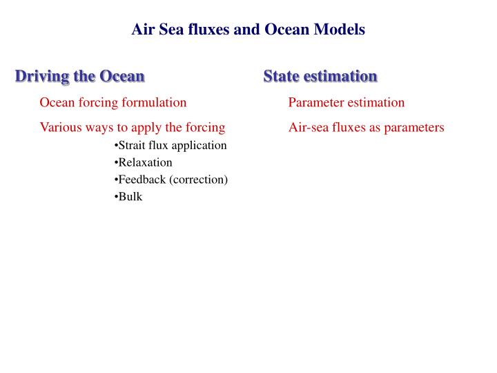
Air Sea fluxes and Ocean Models. Driving the Ocean Ocean forcing formulation Various ways to apply the forcing Strait flux application Relaxation Feedback (correction) Bulk. State estimation Parameter estimation Air-sea fluxes as parameters. Air Sea fluxes driving the Ocean

E N D
Air Sea fluxes and Ocean Models • Driving the Ocean • Ocean forcing formulation • Various ways to apply the forcing • Strait flux application • Relaxation • Feedback (correction) • Bulk • State estimation • Parameter estimation • Air-sea fluxes as parameters
Air Sea fluxes driving the Ocean • Why some sort of flux correction is required
Ocean forcing formulation Just need the wind stress Momentum equation
Ocean forcing formulation Air Sea flux estimates or are necessary at each time step to drive the model Bulk formula and their input parameters T and S equations Penetrating Solar Radiation
Ocean forcing formulation Observed values Ways to apply the forcing Strait flux application The model meridonal heat transport is fully constrained - Model will have no predictive skill on MHT - It usually results in inconsistent model SST (over 40°C in the tropics) ... ... because feedback to the atmosphere is not accounted for
Ocean forcing formulation Ways to apply the forcing Relaxation or nudging to observed values source term is diagnosed Heat flux is zero when observed and model SST agree Flux values and SST are inconsistent
Ocean forcing formulation Ways to apply the forcing Feedback (flux correction) Sensitivity of the Heat Flux to changes in SST (space-time dependent). It is a crude representation of the local effect of the air-sea coupling on the fluxes (feedback term). Obtained from a Taylor expansion of bulk formulas The model meridonal heat transport is prognostic - Model have some predictive skill on MHT - Model SST are realistic
Ocean forcing formulation Ways to apply the forcing Bulk - fluxes are applied strait but: are calculated during model integration with observed atmospheric variables and model prognostic SST. The model meridonal heat transport is prognostic - Model have some predictive skill on MHT - Model SST are realistic
Ocean forcing formulation Ways to apply the forcing The flux correction or the bulk formula are first approaches to coupled A/O GCMs. More sophisticated feedback formulation (non local atmospheric transport) have been formulated. Full GCM coupling is now common for climatye change studies. The coupling between the Oceanic and the Atmospheric model is made through bulk formulas AGCM Surface variables (air temp, humidity, etc..+ radiation boundary conditions Bulk formulas SST, surface currents, ... OGCM
Most used formulations require Bulk formulaFlux correction Flux estimates (radiation)?Flux estimates SST Accurate bulk formulas Accurate bulk formula Atmospheric surface variablesAtmospheric surface variables sea state characteristics Aimed accuracy? A few Wm-2 at interannual time scale to detect climate changes
Air Sea fluxes and Ocean Models • Ocean state estimation • Parameter estimation • Air-sea fluxes as parameters
forcing Q(ti) Initial conditions model solution 1 • 4DVAR modelling system • DM: non linear direct model • TL: tangent linear direct model • AM: adjoin model observations Objective Build a solution of the model which is the closest of the observations Define a cost function J adapted to your problem to be minimised
initial condition model solution at ti Background initial condition flux fields Background flux fields Observations at time ti Project of model solution at time ti at observation point Minimising J means ....
forcing Q(ti) observations model solution 2 Initial conditions model solution 1 • 4DVAR modelling system • DM: non linear direct model • TL: tangent linear direct model • AM: adjoin model Define a cost function J adapted to your problem 1 - Compute TL(or DM) and save full model solution. Input: X0 initial conditions, Q(ti) forcing Output : X(ti) model solution 1 2 - Use AM to bring the gradients of cost function J to zero. Input: X(ti) model solution 1 Output: direction and amplitude of correction applied to selected parameters dX0, dQ(ti) 3 - Use TL to calculate a new solution. Input: X0+ dX0 initial conditions, Q(ti)+dQ(ti) forcing Output : X(ti) model solution 2 Iterate loops 1-2-3 until increment dX dQ < e
forcing Q(ti) observations model solution 2 Initial conditions model solution 1 4DVAR modelling system OUTPUT: A description of the state of the ocean over the assimilation period which is close to consistent to observations. Corrected initial conditions and air-sea fluxes which are consistent with ocean observations over the assimilation period. BUT: Model errors and biases may yields large errors in the increments Many parameters to control simplifications additional errors Do we have the data sets required for the aimed accuracy? (GODDAE)
Air Sea fluxes and Ocean Models • Other data assimilation systems for,ocean state estimation • Optimal interpolation, Kalman filters/smoother/ensemble • Operational system Mecator • European IP Mersea • Not as well suited for parameter estimation but ... • Operational centers produce ocean re-analyses • They have flux requirements for forcing • as for ocean models • need forecast • Assimilation of SST and forcing the model with fluxes ... does it provide a consistent flux correction?