Download
1 / 25
250 likes | 260 Views
Lecture 2: Signals Concepts & Properties. (1) Systems, signals , mathematical models. Continuous-time and discrete-time signals . Energy and power signals . Linear systems. Examples for use throughout the course, introduction to Matlab and Simulink tools

E N D
Lecture 2: Signals Concepts & Properties • (1) Systems, signals, mathematical models. Continuous-time and discrete-time signals. Energy and power signals. Linear systems.Examples for use throughout the course, introduction to Matlab and Simulink tools • Specific objectives for this lecture include • General properties of signals • Energy and power for continuous & discrete-time signals • Signal transformations • Specific signal types • Representing signals in Matlab and Simulink
Lecture 2: Resources • SaS, O&W, Sections 1.1-1.4 • SaS, H&vV, Sections 1.4-1.9 • Mastering Matlab 6 • Mastering Simulink 4
x(t) t x[n] n Reminder: Continuous & Discrete Signals • Continuous-Time Signals • Most signals in the real world are continuous time, as the scale is infinitesimally fine. • E.g. voltage, velocity, • Denote by x(t), where the time interval may be bounded (finite) or infinite • Discrete-Time Signals • Some real world and many digital signals are discrete time, as they are sampled • E.g. pixels, daily stock price (anything that a digital computer processes) • Denote by x[n], where n is an integer value that varies discretely • Sampled continuous signal • x[n] =x(nk)
“Electrical” Signal Energy & Power • It is often useful to characterise signals by measures such as energy and power • For example, the instantaneous power of a resistor is: • and the total energy expanded over the interval [t1, t2] is: • and the average energy is: • How are these concepts defined for any continuous or discrete time signal?
Generic Signal Energy and Power • Total energy of a continuous signal x(t) over [t1, t2] is: • where |.| denote the magnitude of the (complex) number. • Similarly for a discrete time signal x[n] over [n1, n2]: • By dividing the quantities by (t2-t1) and (n2-n1+1), respectively, gives the average power, P • Note that these are similar to the electrical analogies (voltage), but they are different, both value and dimension.
Energy and Power over Infinite Time • For many signals, we’re interested in examining the power and energy over an infinite time interval (-∞, ∞). These quantities are therefore defined by: • If the sums or integrals do not converge, the energy of such a signal is infinite • Two important (sub)classes of signals • Finite total energy (and therefore zero average power) • Finite average power (and therefore infinite total energy) • Signal analysis over infinite time, all depends on the “tails” (limiting behaviour)
Time Shift Signal Transformations • A central concept in signal analysis is the transformation of one signal into another signal. Of particular interest are simple transformations that involve a transformation of the time axis only. • A linear time shift signal transformation is given by: • where b represents a signal offset from 0, and the a parameter represents a signal stretching if |a|>1, compression if 0<|a|<1 and a reflection if a<0.
2p Periodic Signals • An important class of signals is the class of periodic signals. A periodic signal is a continuous time signal x(t), that has the property • where T>0, for all t. • Examples: • cos(t+2p) = cos(t) • sin(t+2p) = sin(t) • Are both periodic with period 2p • NB for a signal to be periodic, the relationship must hold for all t.
Odd and Even Signals • An even signal is identical to its time reversed signal, i.e. it can be reflected in the origin and is equal to the original: • Examples: • x(t) = cos(t) • x(t) = c • An odd signal is identical to its negated, time reversed signal, i.e. it is equal to the negative reflected signal • Examples: • x(t) = sin(t) • x(t) = t • This is important because any signal can be expressed as the sum of an odd signal and an even signal.
Exponential and Sinusoidal Signals • Exponential and sinusoidal signals are characteristic of real-world signals and also from a basis (a building block) for other signals. • A generic complex exponential signal is of the form: • where C and a are, in general, complex numbers. Lets investigate some special cases of this signal • Real exponential signals Exponential growth Exponential decay
Periodic Complex Exponential & Sinusoidal Signals • Consider when a is purely imaginary: • By Euler’s relationship, this can be expressed as: • This is a periodic signals because: • when T=2p/w0 • A closely related signal is the sinusoidal signal: • We can always use: cos(1) T0 = 2p/w0 = p T0 is the fundamental time period w0 is the fundamental frequency
Exponential & Sinusoidal Signal Properties • Periodic signals, in particular complex periodic and sinusoidal signals, have infinite total energy but finite average power. • Consider energy over one period: • Therefore: • Average power: • Useful to consider harmonic signals • Terminology is consistent with its use in music, where each frequency is an integer multiple of a fundamental frequency
General Complex Exponential Signals • So far, considered the real and periodic complex exponential • Now consider when C can be complex. Let us express C is polar form and a in rectangular form: • So • Using Euler’s relation • These are damped sinusoids
Discrete Unit Impulse and Step Signals • The discrete unit impulse signal is defined: • Useful as a basis for analyzing other signals • The discrete unit step signal is defined: • Note that the unit impulse is the first difference (derivative) of the step signal • Similarly, the unit step is the running sum (integral) of the unit impulse.
Continuous Unit Impulse and Step Signals • The continuous unit impulse signal is defined: • Note that it is discontinuous at t=0 • The arrow is used to denote area, rather than actual value • Again, useful for an infinite basis • The continuous unit step signal is defined:
Introduction to Matlab • Simulink is a package that runs inside the Matlab environment. • Matlab (Matrix Laboratory) is a dynamic, interpreted, environment for matrix/vector analysis • User can build programs (in .m files or at command line) C/Java-like syntax • Ideal environment for programming and analysing discrete (indexed) signals and systems
Basic Matlab Operations • >> % This is a comment, it starts with a “%” • >> y = 5*3 + 2^2; % simple arithmetic • >> x = [1 2 4 5 6]; % create the vector “x” • >> x1 = x.^2; % square each element in x • >> E = sum(abs(x).^2); % Calculate signal energy • >> P = E/length(x); % Calculate av signal power • >> x2 = x(1:3); % Select first 3 elements in x • >> z = 1+i; % Create a complex number • >> a = real(z); % Pick off real part • >> b = imag(z); % Pick off imaginary part • >> plot(x); % Plot the vector as a signal • >> t = 0:0.1:100; % Generate sampled time • >> x3=exp(-t).*cos(t); % Generate a discrete signal • >> plot(t, x3, ‘x’); % Plot points
Loops for i=1:100 sum = sum+i; end Goes round the for loop 100 times, starting at i=1 and finishing at i=100 i=1; while i<=100 sum = sum+i; i = i+1; end Similar, but uses a while loop instead of a for loop Decisions if i==5 a = i*2; else a = i*4; end Executes whichever branch is appropriate depending on test switch i case 5 a = i*2; otherwise a = i*4; end Similar, but uses a switch Other Matlab Programming Structures
Matlab Help! • These slides have provided a rapid introduction to Matlab • Mastering Matlab 6, Prentice Hall, • Introduction to Matlab (on-line) • Lots of help available • Type help in the command window or help operator. This displays the help associated with the specified operator/function • Type lookfor topic to search for Matlab commands that are related to the specified topic • Type helpdesk in the command window or select help on the pull down menu. This allows you to access several, well-written programming tutorials. • comp.soft-sys.matlab newsgroup • Learning to program (Matlab) is a “bums on seats” activity. There is no substitute for practice, making mistakes, understanding concepts
Using the Matlab Debugger • Because Matlab is an interpreted language, there is no compile type syntax checking and the likelihood of a run-time error is higher • Run-time debugging can help • Use the debug and breakpoints pull-down menus to determine where to stop program and inspect variables • Step over lines/step into functions to evaluate what happens
Introduction to Simulink • Simulink is a graphical, “drag and drop” environment for building simple and complex signal and system dynamic simulations. • It allows users to concentrate on the structure of the problem, rather than having to worry (too much) about a programming language. • The parameters of each signal and system block is configured by the user (right click on block) • Signals and systems are simulated over a particular time.
Signals in Simulink • Two main libraries for manipulating signals in Simulink: • Sources: generate a signal • Sink: display, read or store a signal
Example: Generate and View a Signal • Copy “sine wave” source and “scope” sink onto a new Simulink work space and connect. • Set sine wave parameters modify to 2 rad/sec • Run the simulation: • Simulation - Start • Open the scope and leave open while you change parameters (sin or simulation parameters) and re-run
Lecture 2: Summary • This lecture has looked at signals: • Power and energy • Signal transformations • Time shift • Periodic • Even and odd signals • Exponential and sinusoidal signals • Unit impulse and step functions • Matlab and Simulink are complementary environments for producing and analysing continuous and discrete signals. • This will require some effort to learn the programming syntax and style!
Lecture 2: Exercises • SaS OW: • Q1.3 • Q1.7-1.14 • Matlab/Simulink • Try out basic Matlab commands on slide 17 • Try creating the sin/scope Simulink simulation on slide 23 and modify the parameters of the sine wave and re-run the simulation • Learning how to use the help facilities in Matlab is important - do it!