Download
1 / 53
670 likes | 1.39k Views
Microstructure-Properties: I Lecture 4A: Mathematical Descriptions of Properties; Magnetic Microstructure. 27-301 Fall, 2002 Prof. A. D. Rollett. Bibliography. De Graef, M., lecture notes for 27-201. Nye, J. F. (1957). Physical Properties of Crystals . Oxford, Clarendon Press.

E N D
Microstructure-Properties: ILecture 4A: Mathematical Descriptions of Properties;Magnetic Microstructure 27-301 Fall, 2002 Prof. A. D. Rollett
Bibliography • De Graef, M., lecture notes for 27-201. • Nye, J. F. (1957). Physical Properties of Crystals. Oxford, Clarendon Press. • Chen, C.-W. (1977). Magnetism and metallurgy of soft magnetic materials. New York, Dover. • Chikazumi, S. (1996). Physics of Ferromagnetism. Oxford, Oxford University Press. • Attwood, S. S. (1956). Electric and Magnetic Fields. New York, Dover. • Newey, C. and G. Weaver (1991). Materials Principles and Practice. Oxford, England, Butterworth-Heinemann. • T. Courtney, Mechanical Behavior of Materials, McGraw-Hill, 0-07-013265-8, 620.11292 C86M. • Kocks, U. F., C. Tomé, et al., Eds. (1998). Texture and Anisotropy, Cambridge University Press, Cambridge, UK. • Reid, C. N. (1973). Deformation Geometry for Materials Scientists. Oxford, UK, Pergamon. • Braithwaite, N. and G. Weaver (1991). Electronic Materials. The Open University, England, Butterworth-Heinemann.
Objective of Lecture 4A • The objective of this lecture is to relate magnetic properties to microstructure as an important example of a non-linear, anisotropic property. This example is illustrated by reference to ferromagnetic materials. In these materials the domain structure provides an additional degree of microstructural complexity that affects properties such as permeability. • The presence of defects (microstructure) in the material has a profound on the magnetic properties of a material. For example, the presence of second phase particles makes a material magnetically hard, just as it makes it mechanically hard.
Mathematical Descriptions • Mathematical descriptions of properties are available. • Mathematics, or a type of mathematics provides a quantitative framework. It is always necessary, however, to make a correspondence between mathematical variables and physical quantities. • In group theory one might say that there is a set of mathematical operations & parameters, and a set of physical quantities and processes: if the mathematics is a good description, then the two sets are isomorphous.
Math of Microstructure-Property Relationships • In order to describe properties, we must first relate a response to a stimulus with a property. • A stimulus is something that one does to a material, e.g. apply a load. • A response is something that is the result of applying a stimulus, e.g. if you apply a load (stress), the material will change shape (strain). • The material property is the connection between the stimulus and the response.
Stimulus PropertyResponse • Mathematical framework for this approach? • The Property is equivalent to a function, P, and the {stimulus, F, response, R} are variables. The stimulus is also called a field because in many cases, the stimulus is actually an applied electrical or magnetic field. • The response is a function of the field:R = R(F) R = P(F)
Scalar, Linear Properties Modulus • In many instances, both stimulus and response are scalar quantities, meaning that you only need one number to prescribe them, so the property is also scalar. • To further simplify, some properties are linear, which means that the response is linearly proportional to the stimulus: R = P F. However, the property is generally dependent on other variables. • Example: elastic stiffness in tension/compression as a function of temperature: R = P(T) F. Temperature
Scalar, non-linear properties • Unfortunately not all properties are linear! • What do we do? In many cases, it useful to expand about a known point (Taylor series). • The response function (property) is expanded about the zero field value, assuming that it is a smooth function and therefore differentiable according to the rules of calculus.
Scalar, non-linear properties, contd. • In the previous expression, the state of the material at zero field is defined by R0which is sometimes zero (e.g. elastic strain in the absence of applied stress) and sometimes non-zero (e.g. in ferromagnetic materials in the absence of an external magnetic field). • Example: magnetization of iron-3%Si alloy, used for transformers [Chen].
Example: magnetization • Magnetization, or B-H curve, in a ferromagnetic material measures the extent to which the atomic scale magnetic moments (atomic magnets, if you like) are aligned. • The stimulus is the applied magnetic field, H, measured in Oersteds (Oe). The response is the Induction, B, measured in kilo-Gauss (kG). • As shown in the plot, the magnetization is a non-linear function of the applied field. Even more interesting is the hysteresis that occurs when you reverse the stimulus. For alternating directions of field, this means that energy is dissipated in the material during each cycle.
Example: magnetization: linearization • An important feature of this example is the possibility of linearization. • How? Take a portion of the property curve and fit a straight line to it. Around H=0, this is the magnetic permeability. B Slope µ permeability H
Example: magnetization: µstructure • How does magnetization depend on microstructure? • In a soft magnetic material, of which Fe-3Si is an example, all the atomic moments are aligned with one another, i.e. the material is fully magnetized. However, there are domains within which all the atomic moments point the same way. The magnetization within each domain, however, points in a different direction. • Generally speaking, domains are smaller than grains. • Anisotropy means that the magnetization within each domain points along a <100> direction.
Magnetism: basics • An elementary understanding of magnetism at the atomic level is assumed. • The basic magnetic properties of a material are often described by a “B-H curve.” • Non-magnetic materials either slightly reject magnetic fields (diamagnetism) or reinforce them (paramagnetism). A limited set of materials (Fe,Co,Ni,Gd and some transition metal oxides) exhibit ferromagnetism, i.e. spontaneous alignment of atomic spins.
Notation BSSaturation flux density/ induction Br Remanence; flux density remaining after applied field is removed HcCoercivity; field required to bring the net flux density to zero. µ Permeability; = B/H c Susceptibility; = M/H µ0 Permeability of free space; 4π.10-7 henry per meter µr Relative permeability, = B/µ0H Ms Saturation magnetization; BS=µ0 Ms WhEnergy lost per cycle; often the most important parameter for a soft magnetic material. BHmax Energy product; often the most important parameter for a hard magnetic material.
Magnetic Domains • A useful exercise is to see how domain walls arise from the anisotropy of magnetism in a ferromagnetic material such as Fe. • The interaction between atomic magnets in Fe is such that the local magnetization at any point is parallel to one of the six <100> directions. [001] [010] _ [100] [100] _ [010] _ [001]
Magnetocrystalline Anisotropy • The fact that different directions magnetize more easily than others in ferromagnetic materials is known as magnetocrystalline anisotropy. This can be measured by applying fields along different directions, e.g. here along 100, 110 and 111 [Chen].
Domains • The local magnetization can point in directions other than a <100> direction, but only if a strong enough external field is applied that can rotate it away from its preferred direction. • Domains are regions in which the local atomic moments all point in the same <100> direction. • At the point (plane, actually) where the local magnetization switches from one <100> direction to another, there is a domain wall.
Magnetization: domains <100> DOMAINS in Fe (Chikazumi);domain walls appear as light anddark lines. GRAINS (Smith); Domains within grains
Magnetic Anisotropy • Why does the magnetization always point along a <100> direction (in Fe)? An over-simple answer is that this is a consequence of the interaction between the atomic moments and that different materials prefer to magnetize along different crystal directions. • An important consequence of this anisotropy is that the local direction of magnetization has to change direction at a grain boundary but this raises the energy of the system. As a result, the domain structure is more complex near the boundary. The next few slides review this effect.
Domain Walls • Since domains of like-oriented moments are volumes like grains, there are (planar) interfaces between domains called domain walls. • Bloch first pointed out that the minimum energy configuration means that the magnetization changes gradually across the wall, 3.10b, not abruptly, 3.10a.
90° Domain Walls • Here is an example of a 90° domain wall. [010] [100]
180° Domain Wall • By contrast, here is a 180° domain wall with the local magnetic moments pointing in opposite directions. [010] [100]
Domain Walls, contd. • In a cubic material with 6 different <100> directions, it is possible to have both 180° walls, and 90° walls. • Domain walls have the lowest energy when they coincide with low index planes (one can say that there is an inclination dependence of the domain wall energy). • Example: in iron, the lowest energy domain walls lie on {001}, {110} and {111}. This explains the way in which the domain walls are straight lines along a small number of directions in the figure. • Just as for grain boundaries, the free energy of a domain wall is always positive.
Grain Boundary Domain Structure • Note how the domain structure, visible as stripes of alternating gray contrast, changes in the vicinity of a grain boundary [Chen].
Demagnetizing Effect (Field) • In a single crystal (no grain boundaries), why does a ferromagnetic material not magnetize in a single direction, with no domains? At the surface of the mono-domain body, there would be free magnetic poles because of the change in magnetization (as for a permanent magnet). A large magnetic field would exist outside the body with which a large amount of (magnetostatic) energy would be associated. By rearranging the internal directions into domains, there is a large reduction in total energy by (near) elimination of the magnetostatic energy.
Hard versus Soft Magnets • We can now understand qualitatively at least, the difference between hard and soft magnets. • In soft magnets, e.g. Fe-3Si, the body has no external field but the domains can be easily brought into alignment with an externally applied field. • In hard magnets, e.g. Alnico, the body does have an external field because the domains have been prevented from changing their alignment.
Hard versus Soft Magnets, contd. • The reasons for some materials being soft and some being hard lie in the microstructure, which we will examine further. In simple terms, soft magnets are single phase and coarse grained: hard magnets are multiphase and fine grained. • There is an important parallel between magnetic and mechanical hardness. The same microstructural features that promote magnetic hardness also promote mechanical hardness.
Changing Domain Structures • There are two ways in which domain structures can change. • A: the domain wall between two domains moves such that the volume of one domain increases and the other decreases. This applies at small fields. • B: the magnetization within a grain rotates (to become aligned with an external field). This only applies at large external fields.
Magnetization Curve • [Chen] The figure below illustrates the difference between the early part of the curve for which domain wall movement is dominant and the later portion where domain rotation dominates. The external field is applied along a non-easy axis (not <100>).
Domain Wall Motion • The process of magnetization can be illustrated with a single crystal example (Fe). Medium field Zero field Low field High field Domainwallmotion Domainrotation Applied field direction
Irreversible Domain Wall Motion • The graph on a previous slide mentioned the “Barkhausen effect” which is observed as a series of jumps in the magnetization curve as the field is increased. • These jumps in magnetization are irreversible - if you take the field off, the domain wall(s) does not make the reverse motion and decrease the net magnetization. • Why the irreversibility?! There are obstacles to domain wall motion that require a certain minimum driving force to force the wall past them. The same barrier exists if you try to force the wall back in the opposite direction. • The barrier is precisely the same as barriers to dislocation motion and in fact, are also precipitates, solute atoms, for example. • This is the basic explanation for magnetic hardness being the same as mechanical hardness.
180° Domain Wall • Moving the domain wall involves “flipping” some of the local magnetic moments to the opposite direction. [010] [100]
Obstacles to domain wall motion • Anything that interacts with a domain wall will make moving it more difficult. For example, a second phase particle will require some extra driving force in order to pull the domain wall past it. Domain wall motion particle
Domain Wall obstacles • A more detailed look at what is going on near particles reveals that magnetostatic energy plays a role in forcing a special domain structure to exist next to a [non-magnetic] particle. Domain wall motion [Electronic Materials]
Particle Pinning of Interfaces • A domain wall is an example of a (planar) interface. • The reason that particles (or voids) exert a pinning effect on domain wall motion (or any other kind of planar defect) is that some of the interfacial area is removed from the system when the interface intersects the particle. This lowers the free energy of the system. In order for the interface to move away from the particle, energy must be put back into the system in order to re-create interfacial area. • Later on (302) we will estimate the energy of domain walls and thus the magnitude of the pinning effect.
Why Domain Walls? • Why should domain walls exist? Answer: because the atomic magnets only like to point in certain directions (as discussed previously). • Can we estimate how much energy it takes to pull a domain away from its preferred direction? Answer: yes, easily. How? Integrate the area under the curve for an easy direction and compare that to the curve for a hard direction. • The area that we need is given by HdM ≈ µ0H2/2. • Think of the difference in areas between the 100 and 111 directions as the difference in energy required to move the crystals of different orientations into the field.
Area under the curve • The area that we need is given by HdM ≈ µ0H2/2. • The energy difference = area(111)-area(100) ≈area(111). 100area 111 area [Chen]
Energy anisotropy estimate: Fe • Area(111) ~4π x 18.105 A.m-1 x 3.104 A.m-1 / 2= 3.4.104 J.m-3 • Compare with the acceptedvalue of the anisotropy coefficient for iron, which is K1 = 4.8 104 J.m-3. • The estimated anisotropy is very close to the measured value! 111 area
How big are domains? • It is reasonable to ask how big domains have to be. One approach to compare the total energy difference for a particle against the available thermal energy. • Total energy for a particle, comparing magnetization in the easy direction (100 in Fe) against the hard direction (111 in Fe) is just the particle volume multiplied by the anisotropy energy (density): E = VK1 = 4πr3/3 K1. • The thermal energy is Ethermal= kT which at room temperature gives Ethermal= 4.10-21J. • Thus the radius at which the energies are similar, for Fe, is: rcritical = 3√{3kT/4πK1} ~ 1.3 nm
Superparamagnetism? • This limiting size, below which we expect a single particle to not have domains because thermal energy can move the magnetization direction around “randomly” is very important technologically. • Small enough particles (relative to the magnetic anisotropy) are called superparamagnetic because they behave like a paramagnetic material even though the bulk form is ferromagnetic. • For magnetic recording, you cannot expect the recording (in the sense of regions of magnetization that remain fixed until the next time you read them) to be stable if thermal energy can change it. • Thus a physical limit exists to the bit density on disks or tapes. • To be safe, the particles need to be much bigger than our estimate - say, 10 times larger.
Magnetocrystalline Anisotropy • The fact that different directions magnetize more easily than others in ferromagnetic materials is known as magnetocrystalline anisotropy. This can be measured by applying fields along different directions, e.g. here along 100, 110 and 111 [Chen].
Labs • Later in the course we will do a lab exercise on imaging domain structures in a sample of Fe-3Si, which is the standard material for manufacturing transformers. We will use cross-polars and rely on the Kerr effect which is where the presence of a magnetic field at the surface of a material rotates the plane of polarization of light. Different directions of magnetization in different domains rotate the polarization differently. This is how the example image of domain structure was obtained.
Application of soft magnetic materials: transformers • A major application of soft magnetic materials is in transformers that step alternating current electrical power up or down in voltage (and therefore current). • The requirement is that a sufficient field is contained within the transformer core, and that it switches each AC cycle with minimal losses (from the hysteresis of the magnetization curve)
Transformer materials, contd. • Other important issues constrain the selection of transformer materials. • Saturation magnetization is a function of atomic species and iron has the highest value for low cost materials. • Silicon is added to iron to raise the resistivity in order to minimize losses. The 3% level represents the maximum that still permits conventional thermomechanical processing (TMP). • Specialized TMP is used to develop near-single-crystal texture, called the Goss texture, {110}<001>.
Supplemental Slides • The following slides contain some useful definitions of terms in magnetism and magnetic materials.
Appendix: Glossary of Magnetism • Ageing: Change in magnetic properties with time, especially in the apparent remanence of a permanent magnet; can be reduced or anticipated by artificial ageing (magnetic, thermal, mechanical). • Air Gap: Space between the poles of a magnet in which there exists a useable magnetic field. • AMR-effect: Non isotropic magneto resistive effect, (see also XMR-effect). • Alnico: Magnet alloys composed of Aluminium, Nickel, Cobalt, Iron and other additives - produced by casting or sintering - can only be processed by grinding. • Alnico P: DIN 17410 designation for plastic bonded Alnico materials. • A/m: amperes per meter : unit of magnetic field strength; 1 A/m= 0,01 A/cm (= 0,01256 Oersted). • Anisotropy: Directional dependence of a physical quantity ; in the case of permanent magnets this relates to remanence, coercivity etc. • Axial magnetization: Magnetization along the symmetric achsis of a bar magnet or along one edge of a block magnet. • B = Induction or flux density: Unit: 1 Tesla = 1 Vs/m2 = 10-4 Vs/cm2 = 104 Gauß. • B (H) Curve: A curve representing the relationship between induction B and field strength H (see also hysteresis loop). • (B • H): Product of the respective induction B and field strength H within a magnet (see also energy density). Unit: 1 J/m3 = 10-3 kJ/m3 = 125,6 Gauß • Oersted = 125,6 • 10-6 MGOe • (B • H)max - Value: Maximum product resulting from B and H on the demagnetization curve, i.e. the largest rectangle which can be drawn within the B (H) curve in the second quadrant of the hysteresis curve; this usually corresponds to the optimal working point. • cgs-units: Physical units which are based on the three fundamental units cm, gram and second (see also SI-units). • CMR-effect: Colossal magneto resistive effect (see also XMR-effect). • Coercive Field Strength Hc, Coercivity: Strength of the demagnetizing field where B = 0 ( HcB ) or J = 0 ( HcJ ). • Columnar crystalline materials: Especially AlNiCo alloys where an orientation of the crystals is formed by a controlled solidification of the melting charge. The material AlNiCo 700 shows a very distinct anisotropy.in contrast to those types where an anisotropy is produced only by applying a magnetic field during heat treatment. • Curie Temperature: The temperature above which the remanence of polarization in a ferro-magnetic material becomes Jr = 0. At all temperatures above the Curie temperature all ferromagnetic materials are paramagnetic. • Demagnetization: Reduction of induction to B = 0; this is obtained practically by the application of an alternating field of decreasing amplitude. • Demagnetization Curve: The second quadrant of the hysteresis loop which is of great importance for permanent magnets. • Demagnetization Factor N: Shape dependent factor which determines the angle between working line and B-axis. N is the tangent of this angle. • Diamagnetism: Magnetic property of materials whose permeability m is smaller than 1, e.g. bismuth. • Dimensional Relationship: Relationship L/D = length / diameter of a bar magnet. For each magnet material the optimal working point corresponds to a fixed L/D value.
Glossary of Magnetism: 2 • Dipole field: first approximation of the field of a magnet at a large distance. The dipole field is defined only by orientation and amount of the magnetic moment and decreases according to 1/r3 with increasing distance r. • Dipole moment: see moment (magnetic) • Eddy current: A current induced in a conductor by a changing magnetic field. It is exploited for example in electricity meters for retarding without any contact. On the other hand it causes losses and undesirable heating in motors, transformers etc. • Effective Flux: Part of the magnetic flux which passes through the air gap. • Energy Density: 1/2 B • H = half of the product resulting from the magnetic induction B and the field strength H (half of the rectangle within the demagnetization curve with its corner at the working point) • Ferromagnetism: Magnetic property of materials with a permeability m >>1, e.g. iron, nickel, cobalt and many of their alloys and compounds. • Field: space having physical properties (see also magnetic field). • Field Constant, Magnetic: m0 = B/H in the vacuum, with m0 = 1,256-10-6 T m / A = 1,256- 10-6 \/s / Am. • Field Line: Means of evident representation of fields. In force fields (e.g. magnetic fields) the tangents to the field lines represent the direction of the effective forces; the density of field lines is a measure of the strength of effective forces. • Field Strength (magnetic) H : a quantitative representation of the strength and the direction (vector) of a magnetic field. Unit 1 A/m = 0,01 A/cm = 0,01256 Oersted. • Flux Density B: No. of field lines per unit of surface. Unit: 1 Tesla = 1 Vs/m2 = 10-4 Vs/cm2 = 104 Gauss. • Flux, magnetic: When a magnetic field is represented by field lines, the total number of lines through a given surface is known as the magnetic flux: measured as an electrical impulse in a coil surrounding this surface on appearance or disappearance of this flux. Unit : 1 Weber (Wb) = 1 Vs = 108 Maxwell. • Fluxmeter: Electronic integrator for measuring a magnetic flux or induction. • Force Line: Visible representation of a force field, especially a magnetic field. • Gauß: Old unit of magnetic induction, 1 Gauß = 10-4 Tesla = 10-8 Vs/cm. • Gaußmeter: Instrument for measuring magnetic induction B. Instruments for measuring magnetic field strength H (Oerstedmeters) are often referred to as Gaußmeters. • Gilbert: Old unit of magnetic tension; 1 Gilbert = 1 Oe cm = 0,796 A. • GMR-effect: Gigantic magneto resistive effect (see also XMR-effect). • H = magnetic field strength, Unit : 1 A/m = 0,01 A/cm = 0,01256 Oe. • Halbach-system: An arrangement of magnets named after the American physicist K. Halbach which produces precise and very homogeneous multipole fields( for example a dipole field) . • Hall probe: Semiconductor probe for measuring magnetic fields (e.g. in an air gap of a magnet system). Hall-probes always are used connected to a gaußmeter.
Glossary of Magnetism: 3 • Hard Ferrite: Term used in DIN 17410 for Oxide magnet materials. • Hard Ferrite P: Term used in DIN 17410 for plastic bonded oxide magnet materials. • Helmholtz-coil: A double coil to produce extremely homogeneous fields. The distance between the two coils is equivalent to their radius. The coil is used for measuring magnetic moments. • Hybrid-material: Plastic bonded material containing several kinds of magnetic powders to adjust certain magnetic properties by using for example Neofer and oxide-powders to reach a predicted price. • Hysteresis - loop: Representation of induction B resp. Polarization J in relation to the magnetizing field strength H. • Induction: 1.The ability of the magnetic field to surround itself with an electric field whilst it is changing. 2.The term induction is also used to mean flux density B. • Induction Constant: See field constant, magnetic. • Isotropy: Equality of physical properties in all directions. • J = magnetic polarization: Density of aligned magnetic moments in a magnetized material Unit 1 T = 1 VS / m2 = 10-4 VS / m2. • Magnetic: Commonly used to denote all materials with noticeably high permeability (especially iron, nickel, cobalt and their alloys); all other materials (gold, brass, copper, wood, stone, etc.) are considered to be non-magnetic. • Magnetic Circuit: Total of parts and gaps through which a magnetic flux passes; in the case of a permanent magnet this consists of the magnet itself, the pole shoes, the air gap and the stray field. • Magnetic Field: Space in which mechanical forces have an effect on magnetic charges or where induction occurs. • Magnetic Field Strength H: See field strength (magnetic). • Magnetic flux: See Flux, magnetic. • Magnetization: 1) The noun arising from "magnetizing” 2) Polarization divided by the magnetic field constant M = J / m0, B = m0 (H+M) = m0 H + J. • Magnetizing: Process of aligning the molecular magnets by an external magnetic field. • Magnetism: Sum of magnetic phenomena as a part of the electromagnetic interaction(force) being one of the four fundamental forces in physics. They are characterized by magnetic field H and magnetic induction B. All the magnetic phenomena are a consequence of moving electric charges (electric currents) whereas electrostatics describes the forces between unmoved electric charges. Electrodynamics finally deals with the connection of electric and magnetic fields varying with time. • With the magnetism of matter an orientation of magnetic moments (colloquial elementary magnets)is defined by polarization J. These moments are composed of the orbital moment of electrons moving around the nucleus of the atom and the so called electron spin moment which is caused by the rotation of the electron around its own axis. If all these moments are compensated the material is called diamagnetic.