Download
1 / 14
290 likes | 1.01k Views
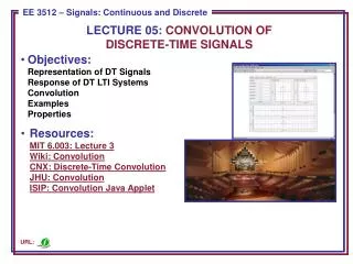
LECTURE 05: CONVOLUTION OF DISCRETE-TIME SIGNALS. Objectives: Representation of DT Signals Response of DT LTI Systems Convolution Examples Properties Resources: MIT 6.003: Lecture 3 Wiki: Convolution CNX: Discrete-Time Convolution JHU: Convolution ISIP: Convolution Java Applet. URL:.

E N D
LECTURE 05: CONVOLUTION OFDISCRETE-TIME SIGNALS • Objectives:Representation of DT SignalsResponse of DT LTI SystemsConvolutionExamplesProperties • Resources:MIT 6.003: Lecture 3Wiki: ConvolutionCNX: Discrete-Time ConvolutionJHU: ConvolutionISIP: Convolution Java Applet URL:
Exploiting Superposition and Time-Invariance DT LTI System • Are there sets of “basic” signals, xk[n], such that: • We can represent any signal as a linear combination (e.g, weighted sum) of these building blocks? (Hint: Recall Fourier Series.) • The response of an LTI system to these basic signals is easy to compute and provides significant insight. • For LTI Systems (CT or DT) there are two natural choices for these building blocks: • Later we will learn that there are many families of such functions: sinusoids, exponentials, and even data-dependent functions. The latter are extremely useful in compression and pattern recognition applications. • CT Systems:(impulse) • DT Systems:(unit pulse)
Response of a DT LTI Systems – Convolution DT LTI • Define the unit pulse response, h[n], as the response of a DT LTI system to a unit pulse function, [n]. • Using the principle of time-invariance: • Using the principle of linearity: • Comments: • Recall that linearity implies the weighted sum of input signals will produce a similar weighted sum of output signals. • Each unit pulse function, [n-k], produces a corresponding time-delayed version of the system impulse response function (h[n-k]). • The summation is referred to as the convolution sum. • The symbol “*” is used to denote the convolution operation. convolution operator convolution sum
LTI Systems and Impulse Response • The output of any DT LTI is a convolution of the input signal with the unit pulse response: • Any DT LTI system is completely characterized by its unit pulse response. • Convolution has a simple graphical interpretation: DT LTI
Visualizing Convolution • There are four basic steps to the calculation: • The operation has a simple graphical interpretation:
Calculating Successive Values • We can calculate each output point by shifting the unit pulse response one sample at a time: • y[n] = 0 for n < ??? • y[-1] = • y[0] = • y[1] = • … • y[n] = 0 for n > ??? • Can we generalize this result?
Graphical Convolution 2 1 -1 -1 1 -1 k = -6 -5 -4 -3 -2 -1 0 1 2 3 4 5 6 7 8 9
Graphical Convolution (Cont.) 2 1 -1 -1 1 -1 k = -6 -5 -4 -3 -2 -1 0 1 2 3 4 5 6 7 8 9
Graphical Convolution (Cont.) • Observations: • y[n] = 0 for n > 4 • If we define the duration of h[n] as the difference in time from the first nonzero sample to the last nonzero sample, the duration of h[n], Lh, is4 samples. • Similarly, Lx = 3. • The duration of y[n] is: Ly = Lx +Lh– 1. This is a good sanity check. • The fact that the output has a duration longer than the input indicates that convolution often acts like a low pass filter and smoothes the signal.
Examples of DT Convolution • Example: delayed unit-pulse • Example: unit-pulse • Example: unit step • Example: integration
Properties of Convolution • Implications • Commutative: • Distributive: • Associative:
Useful Properties of (DT) LTI Systems • Causality: • Stability: Bounded Input ↔ Bounded Output Sufficient Condition: Necessary Condition:
Summary • We introduced a method for computing the output of a discrete-time (DT) linear time-invariant (LTI) system known as convolution. • We demonstrated how this operation can be performed analytically and graphically. • We discussed three important properties: commutative, associative and distributive. • Question: can we determine key properties of a system, such as causality and stability, by examining the system impulse response? • There are several interactive tools available that demonstrate graphical convolution: ISIP: Convolution Java Applet.