Chapter 3: Examining Relationships

1. Chapter 3: Examining Relationships Introduction: Most statistical studies involve more than one variable. In Chapters 1 and 2 we used the boxplot /stem-leaf plot/ histogram to analyze one-variable distributions . In this chapter we will observe studies with two or more variables. • Exploration: SAT Activity - Verbal vs. Math Scores • Consider the following: • Is there an obvious pattern? • Can you describe the pattern? • Can you see any obvious association between SAT Math and SAT Verbal?

2. I. Variables – A. Response – measures an outcome of a study B. Explanatory – attempts to explain the observed outcome Example 3.1 Effect of Alcohol on Body Temperature Alcohol has many effects on the body. One effect is a drop in body temperature. To study this effect, researchers give several different amounts of alcohol to mice, then measure the change in each mouse’s body temperature in the 15 minutes after taking the alcohol. Response Variable – Explanatory Variable – Note: When attempting to predict future outcomes, we are interested in the response variable.

3. In Example 3.1 alcohol actually causes a change in body temperature. Sometimes there is no cause-and-effect relationship between variables. As long as scores are closely related, we can use one to predict the other. • Correlation and Causation

4. Exercise 3.1 Explanatory and Response Variables In each of the following situations, is it more reasonable to simply explore the relationship between the two variables or to view one of the variables as an explanatory variable and the other as a response variable? In the latter case, which is the explanatory variable and which is the response variable? • The amount of time spent studying for a stat test and the grade on the test • The weight and height of a person • The amount of yearly rainfall and the yield of a crop • A student’s grades in statistics and French • The occupational class of a father and of a son

5. a) Time spent studying is explanatory; the grade is the response variable. • (b) Explore the relationship; there is no reason to view one or the other as explanatory. • (c) Rainfall is explanatory; crop yield is the response variable. • (d) Explore the relationship. • (e) The father’s class is explanatory; the son’s class is the response variable.

6. Exercise 3.2 Quantitative and Categorical Variables How well does a child’s height at age 6 predict height at age 16? To find out, measure the heights of a large group of children at age 6, wait until they reach age 16, then measure their heights again. What are the explanatory and response variables here? Are these variables categorical or quantitative? Height at age six is explanatory, and height at age 16 is the response variable. Both are quantitative.

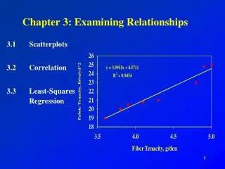
7. 3.1 Scatterplots Scatterplots show the relationship between two quantitative variables taken on the same individual observation. Exercise 3.7 Are Jet Skis Dangerous An article in the August 1997 issue of the Journal of the American Medical Association reported on a survey that tracked emergency room visits at randomly selected hospitals nationwide. Here are data on the number of jet skis in use, the number of accidents, and the number of fatalities for the years 1987 – 1996:

8. Exercise 3.7 Continued • We want to examine the relationship between the number of jet skis in use and the number of accidents. Which is the explanatory variable? • Make a scatter plot of these data. What does the scatterplot show about the relationship between these variables?

9. Interpreting Scatterplots Look for an overall pattern and for striking deviation from that pattern In particular, the direction, form and strength of the relationship between the two variables. a) direction – negative, positive b) form – clustering of data, linear, quadratic, etc. c) strength – how closely the points follow a clear form • Note: in Sec. 3.2 we will discover the value “r” which is a measure of both direction and strength.

10. Positive correlation (direction) – when above average values of one variable tend to accompany above average values of the other variable. Also, the same for below average.

11. Negative correlation (direction) – when above average values of one variable tend to accompany below average values of the other variable. Note: The more students who took the test, the lower the state average- -this is the “open enrollment” concept.

12. No correlation

13. Linear Relationship – when points lie in a straight line pattern.

14. Outliers – in this case, deviations from the overall scatterplot patterns.

15. III. Drawing Scatterplots – Step 1. Scale the horizontal and vertical axes. The intervals MUST be the same. Step 2. Label both axes. Step 3. Adopt a scale that uses the whole grid. Step 4. Add a categorical variable by using a different plotting symbol or color.

16. A scatterplot with categorical data included. III. Example 3.4 pg 127: Heating Degree-Days end Sec. 3.1

17. Sec. 3.2 Correlation ( r ) - is a measure of the direction and strength of the linear relationship between two quantitative variables.

18. Sec. 3.2 Correlation ( r ) Characteristics of “r”- A. Indicates the direction of a linear relationship by its sign B. Always satisfies C. Ignores the distinction between explanatory and response variables D. Requires that both variables be quantitative E. Is not resistant* * herein, correlation joins the mean and standard deviation

19. II. Graphical Interpretations of “r”

20. III. Calculating “r” where,

21. IV. Calculating “r” –Exercise 3.24 page 142. L1 Femur: 38 56 59 64 74 L2Humerus: 41 63 70 72 84

24. end 3.2

25. Exploration: Land-Slide Lab – Preparing for Least-Squares Regression Recall:

26. Sec. 3.3 Least-Squares Regression • Introduction • A. Linear regressionhas many practical uses. Most applications of linear regression fall into one of the following two broad categories: • 1. If the goal is prediction or forecasting linear regression can be used to fit a predictive model to an observed data set of y and X values. After developing such a model, if an additional value of X is then given without its accompanying value of y, the fitted model can be used to make a prediction of the value of y.

27. Linear Regression contd: • 2. Given a variable y and a number of variables X1, ..., Xp that may be related to y, linear regression analysis can be applied to quantify the strength of the relationship between y and the Xj, to assess which Xj may have no relationship with y at all, and to identify which subsets of the Xj contain redundant information about y. • B. Linear regressionmodels are often fitted using the least-squaresapproach, but they may also be fitted in other ways, such as by minimizing the “lack of fit” in some other norm. Conversely, the least squares approach can be used to fit models that are not linear models. Thus, while the terms “least-squares” and linear model are closely linked, they are not synonymous.

28. II. Least-Squares Regression- Summary: The method of least-squaresis a standard approach to the approximate solution of over determined systems (sets of equations in which there are more equations than unknowns). "Least-squares" means that the overall solution minimizes the sum of the squares of the errors made in solving every single equation. The most important application is in data fitting. The best fit in the least-squares sense minimizes the sum of residuals, a residual being the difference between an observed value and the fitted value provided by a model.

29. Simply put, aregression line is a straight line that describes how a response variable y changes as an explanatory variable x changes. A regression line is often used to predict the value of y for a given value of x. Regression, unlike correlation, requires that we have an explanatory variable and a response variable.

30. III. Recall:Correlation (r) makes no use of the distinction between explanatory and response variables. That is, it is not necessary that we define one of the quantitative variables as a response variable and the second as the explanatory variable. It doesn’t matter—for the calculation of rho--which one is the y (D.V.) and which one is x (I.V.). In least-squares regression we are required to designate a response variable (y) and an explanatory variable (x).

31. IV. Regression line– a line that describes how a response variable (y) changes as an explanatory varible (x) changes. A. Regression lines are often used to predict the value of “y” for a given value of “x”. equation of the regression line • “y” is the observed value, is the predicted value of “y”.

32. A household gas consumption data with a regression line for predicting gas consumption from degree-days. • The least-squares line is determined in terms of the means and s.d.’s of the two • variables and their correlation.

33. B. Least-squares regression line of “y” on “x” is the line that makes the sum of the squares of the vertical distances (or, “y’s”) of the data points from the line as small as possible. This minimizes the error in predicting .

34. C. Prediction errors are errors in “y” which is the vertical direction in the scatterplot and are calculated as D. To determine the equation of a least-squares line, (1) solve for the intercept “a” and the slope “b” —thus we have two unknowns. However, it can be shown that every least-squares regression line passes through the point, Next, (2) the slope of the least-squares line is equal to the product of the correlation (rho) and the quotient of the s.d.’s

35. E. Constructing the least-squares equation- Given some explanatory and response variable with the following stat summary - Even though we don’t know the actual data we can till construct the equation and use it to make predictions. The slope and intercept can be calculated as So that the least-squares line has equation

36. Exploration Part II. Complete the Landslide Activity Exploration Part III. LSRL on the calculator pg154

37. We know that the correlation r is the slope of the least-squares regression line when we measure both x and y in standardized units. The square of the correlation is the fraction of the variance of one variable that is explained by least-squares regression on the other variable. When you report a regression, give r-square as a measure of how successful the regression was in explaining the response.

38. While correlation coefficients are normally reported as r = (a value between -1 and +1), squaring them makes then easier to understand. The square of the coefficient (or r-square) is equal to the percent of the variation in one variable that is related to the variation in the other. After squaring r, ignore the decimal point. An r of .5 means 25%of the variation is related (.5 squared =.25). An r value of .7 means 49%of the variance is related (.7 squared = .49).

39. Household gas consumption example - The correlation r = 0.9953 is very strong and r-square = 0.9906. Most of the variation in y is accounted for by the fact that outdoor temperature (measured by degree-days x) was changing and pulled gas consumption along with it. There us only a little remaining variation in y, which appears in the scatter points about the line.

40. V. Summary of Least-Squares Regression- The distinction between explanatory and response variables is essential in regression. B. There is a close relationship between correlation and the slope of the least-squares line. The slope is This means that along the regression line, a change of one s.d. in x corresponds to a change of r standard deviations in y. C. The LSRL always passes through the point on the graph of y against x. D. The correlation describes the strength of the straight-line relationship. In the regression setting, this description takes a specific form: the square of the correlation is the fraction of the variation in the values of y that is explained by the least-squares regression of y on x.

41. VI. Residuals - a residual is the difference between an observed value of the response variable and the value predicted by the regression line. That is, residual = observed y – predicted y A. A residual plot is a scatterplot of the regression residuals against the explanatory variable. These plots assist us in assessing the fit of a regression line. B. Residual example: A study was conducted to test whether the age at which a child begins to talk can be reliably used to predict later scores on a test (taken much later in years) of mental ability—in this instance, the “Gesell Adaptive Score” test. The data appear on in the next slide.

42. Scatterplot of Gesell Adaptive Scores vs the age at first word for 21 kids. The line is the LSRL for predicting Gesell score from age at first word. The plot shows a (-) relationship that is moderately linear, with r = -.640 The residual plot for the regression shows how far the data fall from the regression line. Child 19 is an outlier and child 18 is an “influential” observation that does not have a large residual.

43. Uniform scatter indicates that the regression line fits the data well. The curved pattern means that a straight line in an inappropriate model. The response variable y has more spread for larger values of the explanatory variables x, so the predication will be less accurate when x is larger.

44. C. The residuals from the least-squares line have the special property: the mean of the least-squares residuals is always zero. VI. Influential Observations – an observation is influential for a statistical calculation if removing it would markedly change the result of the calculation. A. Outlier- is an observation that lies outside the overall pattern of other observations. B. Points that are outliers in the x direction of a scatterplot are often influential for the LSRL but need not have large residuals. end Sec. 3.3 and Chpt. 3