Download
1 / 23
230 likes | 345 Views
Chapter 3 Examining Relationships. “Get the facts first, and then you can distort them as much as you please.” Mark Twain. 3.1 Scatterplots. Many statistical studies involve MORE THAN ONE variable.

E N D
Chapter 3Examining Relationships “Get the facts first, and then you can distort them as much as you please.” Mark Twain
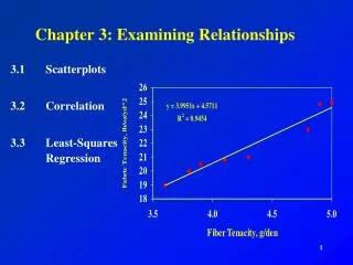
3.1 Scatterplots • Many statistical studies involve MORE THAN ONE variable. • A SCATTERPLOT represents a graphical display that allows one to observe a possible relationship between two quantitative variables.
Response Variable Measures an outcome of a study Explanatory variable Attempts to explain the observed outcomes Response Variable vs. Explanatory Variable
When we think changes in a variable xexplain, or even cause, changes in a second variable, y, we call x an explanatory variable and y a response variable. y Response Variable x Explanatory variable Response Variable vs. Explanatory Variable
IMPORTANT! • Even if it appears that y can be “predicted” from x, it does not follow that x causes y. • ASSOCIATION DOES NOT IMPLY CAUSATION.
When examining a scatterplot, look for an overall PATTERN. • Consider: • Direction • Form • Strength • Positive association • Negative association • outliers
Positive Association (between two variables) Above-average values of one tend to accompany above-average values of the other Below-average values of one tend to accompany below-average values of the other Negative Association (between two variables) Above-average values of one tend to accompany below-average values of the other Positive vs. Negative Association
3.2 Correlation • Describes the direction and strength of a straight-line relationship between two quantitative variables. • Usually written as r.
Facts About Correlation • Positive r indicates positive association between the variables and negative r indicates negative association. • The correlation r always fall between –1 an 1 inclusive. • The correlation between x and y does NOT change when we change the units of measurement of x, y, or both. • Correlation ignores the distinction between explanatory and response variables. • Correlation measures the strength of ONLY straight-line association between two variables. • The correlation is STRONGLY affected by a few outlying observations.
3.3 Least-Squares Regression • If a scatterplot shows a linear relationship between two quantitative variables, least-squares regression is a method for finding a line that summarizes the relationship between the two variables, at least within the domain of the explanatory variable x. • The least-squares regression line (LSRL) is a mathematical model for the data.
Regression Line • Straight line • Describes how a response variable y changes as an explanatory variable x changes. • Sometimes it is used to PREDICT the value of y for a given value of x. • Makes the sum of the squares of the vertical distances of the data points from the line as small as possible.
Residual • A difference between an OBSERVED y and a PREDICTED y:
Some Important Facts About the LSRL • It is a mathematical model for the data. • It is the line that makes the sum of the squares of the residuals AS SMALL AS POSSIBLE. • The point is on the line, where is the mean of the x values, and is the mean of the y values. • The form is (N.B. b is the slope and a is the y-intercept. (On the regression line, a change of one standard deviation in x corresponds to a change of r standard deviations in y)
Some Important Facts About the LSRL • The slope b is the approximate change in y when x increases by 1. • The y-intercept a is the predicted value of y when
Coefficient of Determination • Symbolism: • It is the fraction of the variation in the values of y that is explained by the least-squares regression of y on x. • Measure of HOW SUCCESSFUL the regression is in explaining the response.
Things to Note: • Sum of deviations from mean = 0. • Sum of residuals = 0. • r2 > 0 does not mean r > 0. If x and y are negatively associated, then r < 0.
Outlier • A point that lies outside the overall pattern of the other points in a scatterplot. • It can be an outlier in the x direction, in the y direction, or in both directions.
Influential Point • A point that, if removed, would considerably change the position of the regression line. • Points that are outliers in the x direction are often influential.
Words of Caution • Do NOT CONFUSE the slope b of the LSRL with the correlation r. • The relation between the two is given by the formula • If you are working with normalized data, then b does equal r since • When you normalize a data set, the normalized data has a mean = 0 and standard deviation = 0.
More Words of Caution • If you are working with normalized data, the regression line has the simple form • Since the regression line contains the mean of x and the mean of y, and since normalized data has a mean of 0, the regression line for normalized x and y values contains (0, 0).