Download
1 / 25
290 likes | 485 Views
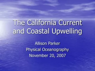
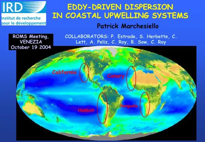
EDDY-DRIVEN DISPERSION IN COASTAL UPWELLING SYSTEMS. Patrick Marchesiello. COLLABORATORS: P. Estrade, S. Herbette, C. Lett, A. Peliz, C. Roy, B. Sow, C. Roy. ROMS Meeting, VENEZIA October 19 2004. California. Canary. Benguela. Humbolt. Coastal Upwelling?.

E N D
EDDY-DRIVEN DISPERSION IN COASTAL UPWELLING SYSTEMS Patrick Marchesiello COLLABORATORS: P. Estrade, S. Herbette, C. Lett, A. Peliz, C. Roy, B. Sow, C. Roy ROMS Meeting, VENEZIA October 19 2004 California Canary Benguela Humbolt
Coastal upwelling Retention zone Eddy mixing zone Divergence zone Marchesiello et al., 2003 Mitchum & Clark, 1978 Lentz & Austin, 2002
ROMS_AGRIF http://www.ird.brest.fr/Roms_tools • ROMS: HYDRODYNAMIC MODEL optimized for regional and coastal high resolution, multi-scale, multidisciplinary applications • AGRIF: Online, synchronous nesting method (L. Debreu) • ROMS_TOOL: Pre- and post-processing package (P. Penven) • DIAGNOSTIC TOOLS:Lagrangian tracers, budgets … • APPLICATION MODELS:Ecosystem dynamics, Water quality, Sediment transport
Note on Regional Models POG - 0.25 deg ROMS – 0.25 deg
APPLICATION TO THE CALIFORNIA CURRENT SYSTEM: CONFIGURATION AND STRATEGY Volume Averaged KE (cm2/s2) 20km, 10km, 5km 20km, 10km, 5km, 2.5km Surface Averaged KE (cm2/s2) • Nesting of the inner domain: on-line or off-line. • Model integration: 10 years. • Surface and lateral boundary forcing: Monthly climatologies.
SST - Model SST - AVHRR Mesoscale Variability in the CCS • Marchesiello et al. (JPO, 2003) • Realistic simulation of the Coastal Transition Zone • More than 2/3 of the mesoscale variability is intrinsic, and produced through instabilities (baroclinic and barotropic) of the coastal currents generated in the upwelling process.
Drifter Estimation [180] 100 Eddy Kinetic Energy [cm2/s2] Model Resolution [km] 10 1 5 10 20 Model Convergence
Canary Current System Configuration Mercator ROMS – Sahara 5 km ROMS – Canary 25 km Levitus C. Blanc C. Blanc Clipper C. Vert
Sahara California 20 17 26 8
Mesoscale Activity In California and Canary Systems California Model Sahara SSH Standard Deviation [cm] For non-seasonal variability
Mesoscale Activity In California and Canary Systems California Model Sahara SSH Standard Deviation [cm] For non-seasonal variability California Altimetry Sahara Topex/ERS from AVISO
Wind Forcing California Morocco Units: Pascal
BAROCLINICITY: Two layer approach • The upwelling front • results from upwelling of the thermocline (Mooers et al., 1976) • Baroclinic instability: • energy conversion from available potential energy to eddy kinetic energy • varies with vertical shear of velocity (Pedlosky, 1986; Barth, 1989) • U=(g’H0)1/2 • where g’=g(ρ2-ρ1)/ ρ2
JOINT I cruise, after Huyer(1976) Salinity profiles & Reduced Gravity Salinity relative to surface Temperature relative to surface Potential density • California • g’=0.019 • Canary • g’=0.008 California California Canary Canary
T’u’ = -Kx dT/dx MESOSCALE CROSS-SHORE DIFFUSION T Erosion of coastal properties Mixing 500km 100km Offshore distance X100 m2/s • Swenson and Niiler (1996)from drifting-buoy trajectories, 1985-1988: K = 1.1 - 4.6 103 m2/s with higher values for Kx compared to Ky • Model: Kx = 2.3 103 m2/s and Ky = 1.3 103 m2/s
Ammonium Nitrate Chlorophyll A Phytoplankton Zooplankton Large Detritus Small Detritus THE ECOSYSTEM MODEL HYDRODYNAMICS Upwelling Nitrification Light Transport New Prod. Reg. Prod. Grazing Breakdown Mortality Excretion Aggregation Sink
New Production NO3 transport Spring-time biology fluxes Units: mmol N cm-2 a-1 LINEAR MODEL (advection terms turned off in the momentum equation) NON-LINEAR MODEL
Seawifs Annual Chl Retention Map From Lagrangian Study SSH Standard Deviation
BIOLOGICALLY ACTIVE AREA IN UPWELLING SYSTEMS CANARY PERU-CHILI BENGUELA CALIFORNIA What drives the observeddifferences in cross-shore distribution of physical and biogeochemical properties? • Latitude (solar flux) • Fe depositions from Sahara (Lene et al., 2001) • Shelf width & nutrients (Johnson et al., 1997) • Mesoscale physics(Marchesiello et al., 2003)