Download
1 / 19
190 likes | 280 Views
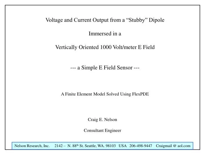
Voltage and Current Output from a “Stubby” Dipole Immersed in a Vertically Oriented 1000 Volt/meter E Field --- a Simple E Field Sensor --- A Finite Element Model Solved Using FlexPDE. Craig E. Nelson Consultant Engineer. Background:

E N D
Voltage and Current Output from a “Stubby” Dipole Immersed in a Vertically Oriented 1000 Volt/meter E Field --- a Simple E Field Sensor --- A Finite Element Model Solved Using FlexPDE Craig E. Nelson Consultant Engineer
Background: A “stubby” dipole antenna may be used as an electrostatic field sensor. For a long time I have been interested in knowing the extent to which such an antenna sensor will distort the electric field within which it is immersed. The following numerical experiment provides results for one simple physical situation. No attempt at sensor optimization has been made. Many further extensions of this experiment are easily possible.
Problem Geometry and Physical Layout of the Solution Domain
1000 Volts/meter E Field Copper Rod Length = 20 cm Radius = 5 cm Conductivity = 5.99e7 Vout Plus Iout Hi Resistance Rod Length = 10 cm Radius = 5 cm Conductivity = 6.36e-7 Vout Copper Rod Length = 20 cm Radius = 5 cm Conductivity = 5.99e7 Vout Minus 1000 Volts/meter E Field 3-D Sensor Physical Layout
1000 Volt/meter E Field “Stubby” Dipole Centerline Solution Domain (cylindrical Geometry)
The Partial Differential Equation to be Solved is: div ( J ) = 0 in cylindrical (r,z) coordinates: div ( J ) = (1/r)*dr( r*Jr)+ dz( Jz) = 0 where: Jr=cond*Er Jz=cond*Ez J=vector( Jr,Jz ) Jm=magnitude(J) Jr and Jz are the current densities in the r and z directions (amps/meter^2) and: Er= -dr(U) Ez=-dz(U) E=-grad(U) Em=magnitude(E) Er and Ez are the electric field strength in the r and z directions (volts/meter) and: cond = conductivity in the different solution sub domains (siemens/meter) The Boundary Conditions are: Natural (U) = 0 on the centerline and domain outer wall (Neuman) Value (U) = FieldStrength*Hdomain/2 on the top surface (Dirichlet) Value (U) = - FieldStrength*Hdomain/2 on the bottom surface (Dirichlet) where: U is the potential (volts) and: Fieldstrength and Hdomain are given parameters note: dr(J) = d(J) / d(r) dz(U) = d(U) / d(z) and so on
Contour Plot of Potential (referenced to the load resistance vertical axis center)
Contour Plot of Potential (referenced to the load resistance vertical axis center)
Contour Plot of log base 10 of Electric Field Strength (three = 1000 volts/meter)
Plot of Potential along the Solution Domain Centerline (volts)
Plot of Electrical Field Strength Magnitude along the Solution Domain Centerline (volts/meter)
Plot of log base 10 of Electrical Field Strength Magnitude along the Solution Domain Centerline (zero = 1 volt/meter)
Summary and Conclusions: A numerical experiment analysis of a “stubby” dipole antenna electric field sensor has been accomplished. The analysis shows that the despite a moderately high electric field strength of 1000 volts/meter, the sensor output voltage and current are rather small. Apparently only a few tens of micro volts appear across the resistive load (upper to lower terminal resistance given as 10 megohm) with a load current flow of several pico-amps. This is because the highly conducting copper dipole arms “short” the electrical field to near zero in regions close to the conductors. It would seem that this particular configuration is far from optimal. Many other configurations are possible and could be analyzed by the method presented here