Download
1 / 14
1k likes | 2.92k Views
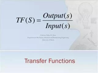
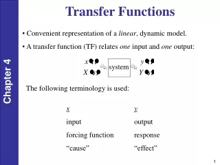
Transfer Functions. Zero-State Response. Linear constant coefficient differential equation Input x ( t ) and output Zero-state response: all initial conditions are zero

E N D
Zero-State Response • Linear constant coefficient differential equation Input x(t) and output Zero-state response: all initial conditions are zero Laplace transform both sides of differential equation with all initial conditions being zero and solve for Y(s)/X(s)
Transfer Function • H(s) is called the transfer function because it describes how input is transferred to the output in a transform domain (s-domain in this case) Y(s) = H(s) X(s) y(t) = L-1{H(s) X(s)} = h(t) * x(t) H(s) = L{h(t)} • Transfer function is Laplace transform of impulse response
Laplace transform Assume input x(t) and output y(t) are causal Ideal delay of T seconds Initial conditions (initial voltages in delay buffer) are zero y(t) x(t) Transfer Function Examples
Ideal integrator with y(0-) = 0 Ideal differentiator with x(0-) = 0 y(t) x(t) Transfer Function Examples y(t) x(t)
x(t) x(t) s 1/s X(s) s X(s) X(s) Cascaded Systems • Assume input x(t) and output y(t) are causal • Integrator first,then differentiator • Differentiator first,then integrator • Common transfer functions A constant (finite impulse response) A polynomial (finite impulse response) Ratio of two polynomials (infinite impulse response) x(t) x(t) 1/s s X(s) X(s)/s X(s)
X(s) W(s) H(s) Y(s) X(s) H1(s) H2(s) Y(s) = X(s) H1(s)H2(s) Y(s) H1(s) = X(s) Y(s) X(s) H1(s) + H2(s) Y(s) H2(s) E(s) X(s) G(s) 1 + G(s)H(s) Y(s) X(s) G(s) Y(s) = - H(s) Block Diagrams
X(s) X(s) H1(s) H2(s) H1(s) H2(s) Y(s) Y(s) H1(s) = X(s) Y(s) X(s) H1(s) + H2(s) Y(s) H2(s) Cascade and Parallel Connections • Cascade W(s) = H1(s) X(s) Y(s) = H2(s)W(s) Y(s) = H1(s) H2(s) X(s) Y(s)/X(s) = H1(s)H2(s) One can switch the order of the cascade of two LTI systems if both LTI systems compute to exact precision • Parallel Combination Y(s) = H1(s)X(s) + H2(s)X(s) Y(s)/X(s) = H1(s) + H2(s)
Governing equations Combining equations What happens if H(s) is a constant K? Choice of K controls all poles in transfer function Common LTI system in EE362K Introduction to Automatic Control andEE445L Microcontroller Applications/Organization E(s) F(s) G(s) 1 + G(s)H(s) Y(s) F(s) G(s) Y(s) = - H(s) Feedback Connection
External Stability Conditions • Bounded-input bounded-output stability Zero-state response given by h(t) * x(t) Two choices: BIBO stable or BIBO unstable • Remove common factors in transfer function H(s) • If all poles of H(s) in left-hand plane, All terms in h(t) are decaying exponentials h(t) is absolutely integrable and system is BIBO stable • Example: BIBO stable but asymptotically unstable Based on slide by Prof. Adnan Kavak
Internal Stability Conditions • Stability based on zero-input solution • Asymptotically stable if and only if Characteristic roots are in left-hand plane (LHP) Roots may be repeated or non-repeated • Unstable if and only if (i) at least characteristic root in right-hand plane and/or (ii) repeated characteristic roots are on imaginary axis • Marginally stable if and only if There are no characteristic roots in right-hand plane and Some non-repeated roots are on imaginary axis Based on slide by Prof. Adnan Kavak
est h(t) y(t) Frequency-Domain Interpretation • y(t) = H(s) e s tfor a particular value of s • Recall definition offrequency response: ej 2p f t h(t) y(t)
Frequency-Domain Interpretation • Generalized frequency: s = s + j 2 p f • We may convert transfer function into frequency response by if and only if region of convergence of H(s) includes the imaginary axis • What about h(t) = u(t)? We cannot convert H(s) to a frequency response However, this system has a frequency response • What about h(t) = d(t)?
Lowpass filter Highpass filter Bandpass filter Bandstop filter Frequency Selectivity in Filters |Hfreq(f)| |Hfreq(f)| 1 1 f f |Hfreq(f)| |Hfreq(f)| f f Linear time-invariant filters are BIBO stable