Download
1 / 14
140 likes | 145 Views
Lecture 16: Continuous-Time Transfer Functions. 6 Transfer Function of Continuous-Time Systems (3 lectures): Transfer function, frequency response, Bode diagram. Physical realisability, stability. Poles and zeros, rubber sheet analogy. Specific objectives for today:

E N D
Lecture 16: Continuous-Time Transfer Functions • 6 Transfer Function of Continuous-Time Systems (3 lectures): Transfer function, frequency response, Bode diagram. Physical realisability, stability. Poles and zeros, rubber sheet analogy. • Specific objectives for today: • Transfer functions and frequency response • Bode diagrams
Lecture 16: Resources • Core material • SaS, O&W, C6.1, 6.2, 9.7 • Background material • MIT Lectures 9, 12 and 19
Introduction: Transfer Functions & Frequency Response • We can use the Fourier (Laplace) transfer function H(jw) (H(s)) in a variety of ways: • Design a system/filter with appropriate frequency domain characteristics • Calculate the system’s time domain response using Y(jw)=H(jw)X(jw) and taking the inverse Fourier transform • However, we can also get a lot of information from studying H(jw) directly and representing it in polar fashion as • H(jw) = |H(jw)|ejH(jw) H(s) x(t) y(t)
Example: 1st Order System and Cos Input • The 1st order system transfer function is: (a>0, h(t)=e-atu(t)) • The input signal x(t)=cos(w0t), which has fundamental frequency w0, has Fourier transform: • The (stable) system’s output is:
System Transient & Steady State Response • Compare with the example from lecture 14 • which was solved using the Laplace transform • This is composed of two parts: • Transient (blue) and steady state/natural (green -Fourier) responses
System Gain and Phase Shift • In the frequency domain, the effect of the system on the input signal for the frequency component w is: • Y(jw) = |H(jw)|ejH(jw) |X(jw)|ejX(jw) • |Y(jw)| = |H(jw)||X(jw)| • Y(jw) = H(jw) + X(jw) • The effect of a system, H(jw), has on the Fourier transform of an input signal is to: • Scale the magnitude by |H(jw)|. This is commonly referred to as the system gain. • Shift the phase of the input signal by adding H(jw) to it. This is commonly referred to as the phase shift. • These modifications (magnitude and phase distortions) may be desirable/undesirable and must be understood in system analysis and design.
Example: Cos Input to a 1st Order System • Consider a sinusoidal input signal to a first order, LTI, stable system • When w0 is close to zero, its magnitude is passed on scaled by 1/a • When the |w0| is high, the signal is substantially suppressed • i.e. it is a low pass filter … Magnitude plot (even) Phase plot (odd) We deduce the properties solely by looking at the transfer function in the frequency domain
The Effect of Phase … • The effect of the transfer function’s magnitude is fairly easy to see – it magnifies/suppresses the input signal • The effect of the change in phase is a bit less obvious to imagine. • Consider when the phase shift is a linear function of w: • This system corresponds to a pure time shift of the input (see lectures 7,9,14) • y(t) = x(t-t0) • Slope of the phase corresponds to the time delay • When the phase is not a linear function, it is slightly more complex
Log-Magnitude and Phase Plots • When analysing system responses, it is typical to use a log scaling for the magnitude • log(|Y(jw)|) = log(|H(jw)|) + log(|X(jw)|) • So the gain effect is additive: 0 means “no change” • If the log magnitude is plotted, the effect can be interpreted as adding each individual component (like the time-delayed phase) • Often units are decibels (dB) 20log10 • Similarly, taking logs of frequency allows us to view detail over a much greater range (which is important for frequency selective filters) • Note that taking a log of the frequency, we typically only consider positive frequency values (as the magnitude is even, and the phase is odd)
Bode Plots • A Bode Plot for a system is simply plots of log magnitude and phase against log frequency • Both the log magnitude and phase effects are now additive • Widely used for analysis and design of filters and controllers • Example • Low pass, unity filter Log mag v log freq Phase v log freq
Example 1: Bode Plot 1st Order System • Consider a LTI first order system described by: • Fourier transfer function is: • the impulse response is: • and the step response is: • Bode diagrams are shown as log/log plots on the x and y axis with t=2.
Example 2: Bode Plot 2nd Order System step response(t) • The LTI 2nd order differential equation • which can represent the response of mass-spring systems and RLC circuits, amongst other things • wn is the undamped natural frequency • z is the damping ratio wn=1 z=[0.01 0.1 0.4 1 1.5]
Lecture 16: Summary • A frequency domain analysis of the transfer function/Fourier transform is an important design/analysis concept • It can be understood in terms of • |H(jw)| - magnitude of the Fourier transform of the impulse response (transfer function) • H(jw) – phase of the Fourier transform of the impulse response (transfer function) • Bode plots are plots of log magnitude and phase against log frequency. • Used to plot a greater range of frequencies • Used to plot decibel-type information • Transfer function is now “additive”
Exercises • Theory • Verify the magnitude and phase plots on slide 7 by evaluating the 1st order transfer function for specific values of w (=0, 1, 3, 5, 10), for a=1&10. • SaS, O&W, Q6.15, 6.18, 6.19, 6.27 & 6.28 (use Matlab for “sketching”) • Matlab • 1. Use Simulink to verify the transient/steady state response of a first order system described on Slide 5. • 2. To perform a Bode plot of a first order system (slide 11), • Where t=2 • >> fbode([1], [2 1]); • Type help fbode to find out about the general structure. • Try doing a Bode plot for different values of the decay constant, say 1 and 100, what are the differences? • To perform a Bode plot of the second order system (slide 12) • >> fbode([1], [1 2 1]); • Again, try different values for the differential equation coeffs.