Download

1 / 35
350 likes | 545 Views
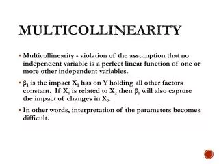
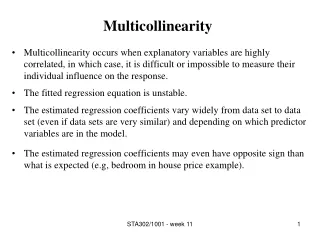
Multicollinearity. Multicollinearity. Multicollinearity (or intercorrelation ) exists when at least some of the predictor variables are correlated among themselves. In observational studies, multicollinearity happens more often than not.

E N D
Multicollinearity • Multicollinearity (or intercorrelation) exists when at least some of the predictor variables are correlated among themselves. • In observational studies, multicollinearity happens more often than not. • So, we need to understand the effects of multicollinearity on regression analyses.
Example #1 n = 20 hypertensive individuals p-1 = 6 predictor variables
Example #1 BP Age Weight BSA Duration Pulse Age 0.659 Weight 0.950 0.407 BSA 0.866 0.378 0.875 Duration 0.293 0.344 0.201 0.131 Pulse 0.721 0.619 0.659 0.465 0.402 Stress 0.164 0.368 0.034 0.018 0.312 0.506 Blood pressure (BP) is the response.
x1x2y 2 5 52 2 5 43 2 7 49 2 7 46 4 5 50 4 5 48 4 7 44 4 7 43 Pearson correlation of x1 and x2 = 0.000 What is effect on regression analyses if predictors are perfectly uncorrelated?
Regress Y on X1 The regression equation is y = 48.8 - 0.63 x1 Predictor Coef SE Coef T P Constant 48.750 4.025 12.11 0.000 x1 -0.625 1.273 -0.49 0.641 Analysis of Variance Source DF SS MS F P Regression 1 3.13 3.13 0.24 0.641 Error 6 77.75 12.96 Total 7 80.88
Regress Y on X2 The regression equation is y = 55.1 - 1.38 x2 Predictor Coef SE Coef T P Constant 55.125 7.119 7.74 0.000 x2 -1.375 1.170 -1.17 0.285 Analysis of Variance Source DF SS MS F P Regression 1 15.13 15.13 1.38 0.285 Error 6 65.75 10.96 Total 7 80.88
Regress Y on X1 and X2 The regression equation is y = 57.0 - 0.63 x1 - 1.38 x2 Predictor Coef SE Coef T P Constant 57.000 8.486 6.72 0.001 x1 -0.625 1.251 -0.50 0.639 x2 -1.375 1.251 -1.10 0.322 Analysis of Variance Source DF SS MS F P Regression 2 18.25 9.13 0.73 0.528 Error 5 62.63 12.53 Total 7 80.88 Source DF Seq SS x1 1 3.13 x2 1 15.13
Regress Y on X2 and X1 The regression equation is y = 57.0 - 1.38 x2 - 0.63 x1 Predictor Coef SE Coef T P Constant 57.000 8.486 6.72 0.001 x2 -1.375 1.251 -1.10 0.322 x1 -0.625 1.251 -0.50 0.639 Analysis of Variance Source DF SS MS F P Regression 2 18.25 9.13 0.73 0.528 Error 5 62.63 12.53 Total 7 80.88 Source DF Seq SS x2 1 15.13 x1 1 3.13
If predictors are perfectly uncorrelated, then… • You get the same slope estimates regardless of the first-order regression model used. • That is, the effect on the response ascribed to a predictor doesn’t depend on the other predictors in the model.
If predictors are perfectly uncorrelated, then… • The sum of squares SSR(X1) is the same as the sequential sum of squares SSR(X1|X2). • The sum of squares SSR(X2) is the same as the sequential sum of squares SSR(X2|X1). • That is, the marginal contribution of one predictor variable in reducing the error sum of squares doesn’t depend on the other predictors in the model.
Same effects for “real data” with nearly uncorrelated predictors? BP Age Weight BSA Duration Pulse Age 0.659 Weight 0.950 0.407 BSA 0.866 0.378 0.875 Duration 0.293 0.344 0.201 0.131 Pulse 0.721 0.619 0.659 0.465 0.402 Stress 0.164 0.368 0.034 0.018 0.312 0.506
Regress BP on Stress The regression equation is BP = 113 + 0.0240 Stress Predictor Coef SE Coef T P Constant 112.720 2.193 51.39 0.000 Stress 0.02399 0.03404 0.70 0.490 S = 5.502 R-Sq = 2.7% R-Sq(adj) = 0.0% Analysis of Variance Source DF SS MS F P Regression 1 15.04 15.04 0.50 0.490 Error 18 544.96 30.28 Total 19 560.00
Regress BP on BSA The regression equation is BP = 45.2 + 34.4 BSA Predictor Coef SE Coef T P Constant 45.183 9.392 4.81 0.000 BSA 34.443 4.690 7.34 0.000 S = 2.790 R-Sq = 75.0% R-Sq(adj) = 73.6% Analysis of Variance Source DF SS MS F P Regression 1 419.86 419.86 53.93 0.000 Error 18 140.14 7.79 Total 19 560.00
Regress BP on BSA and Stress The regression equation is BP = 44.2 + 34.3 BSA + 0.0217 Stress Predictor Coef SE Coef T P Constant 44.245 9.261 4.78 0.000 BSA 34.334 4.611 7.45 0.000 Stress 0.02166 0.01697 1.28 0.219 Analysis of Variance Source DF SS MS F P Regression 2 432.12 216.06 28.72 0.000 Error 17 127.88 7.52 Total 19 560.00 Source DF Seq SS BSA 1 419.86 Stress 1 12.26
Regress BP on Stress and BSA The regression equation is BP = 44.2 + 0.0217 Stress + 34.3 BSA Predictor Coef SE Coef T P Constant 44.245 9.261 4.78 0.000 Stress 0.02166 0.01697 1.28 0.219 BSA 34.334 4.611 7.45 0.000 Analysis of Variance Source DF SS MS F P Regression 2 432.12 216.06 28.72 0.000 Error 17 127.88 7.52 Total 19 560.00 Source DF Seq SS Stress 1 15.04 BSA 1 417.07
If predictors are nearlyuncorrelated, then… • You get similar slope estimates regardless of the first-order regression model used. • The sum of squares SSR(X1) is similar to the sequential sum of squares SSR(X1|X2). • The sum of squares SSR(X2) is similar to the sequential sum of squares SSR(X2|X1).
What happens if the predictor variables are highly correlated? BP Age Weight BSA Duration Pulse Age 0.659 Weight 0.950 0.407 BSA 0.866 0.378 0.875 Duration 0.293 0.344 0.201 0.131 Pulse 0.721 0.619 0.659 0.465 0.402 Stress 0.164 0.368 0.034 0.018 0.312 0.506
Regress BP on Weight The regression equation is BP = 2.21 + 1.20 Weight Predictor Coef SE Coef T P Constant 2.205 8.663 0.25 0.802 Weight 1.200930.09297 12.92 0.000 S = 1.740 R-Sq = 90.3% R-Sq(adj) = 89.7% Analysis of Variance Source DF SS MS F P Regression 1 505.47 505.47 166.86 0.000 Error 18 54.53 3.03 Total 19 560.00
Regress BP on BSA The regression equation is BP = 45.2 + 34.4 BSA Predictor Coef SE Coef T P Constant 45.183 9.392 4.81 0.000 BSA 34.4434.690 7.34 0.000 S = 2.790 R-Sq = 75.0% R-Sq(adj) = 73.6% Analysis of Variance Source DF SS MS F P Regression 1 419.86 419.86 53.93 0.000 Error 18 140.14 7.79 Total 19 560.00
Regress BP on BSA and Weight The regression equation is BP = 5.65 + 5.83 BSA + 1.04 Weight Predictor Coef SE Coef T P Constant 5.653 9.392 0.60 0.555 BSA 5.8316.063 0.96 0.350 Weight 1.03870.1927 5.39 0.000 Analysis of Variance Source DF SS MS F P Regression 2 508.29 254.14 83.54 0.000 Error 17 51.71 3.04 Total 19 560.00 Source DF Seq SS BSA 1 419.86 Weight 1 88.43
Regress BP on Weight and BSA The regression equation is BP = 5.65 + 1.04 Weight + 5.83 BSA Predictor Coef SE Coef T P Constant 5.653 9.392 0.60 0.555 Weight 1.03870.1927 5.39 0.000 BSA 5.8316.063 0.96 0.350 Analysis of Variance Source DF SS MS F P Regression 2 508.29 254.14 83.54 0.000 Error 17 51.71 3.04 Total 19 560.00 Source DF Seq SS Weight 1 505.47 BSA 1 2.81
Effect #1 of multicollinearity When predictor variables are correlated, the regression coefficient of any one variable depends on which other predictor variables are included in the model.
Even correlated predictors not in the model can have an impact! • Regression of territory sales on territory population, per capita income, etc. • Against expectation, coefficient of territory population was determined to be negative. • Competitor’s market penetration, which was strongly positively correlated with territory population, was not included in model. • But, competitor kept sales down in territories with large populations.
Effect #2 of multicollinearity When predictor variables are correlated, the marginal contribution of any one predictor variable in reducing the error sum of squares varies, depending on which other variables are already in model. SSR(X1) = 505.47 SSR(X1|X2) = 88.43 SSR(X2) = 419.86 SSR(X2|X1) = 2.81
Effect #3 of multicollinearity When predictor variables are correlated, the precision of the estimated regression coefficients decreases as more predictor variables are added to the model.
What is the effect on estimating mean or predicting new response?
Weight Fit SE Fit 95.0% CI 95.0% PI 92 112.70.402 (111.85,113.54) (108.94,116.44) BSA Fit SE Fit 95.0% CI 95.0% PI 2 114.10.624 (112.76,115.38) (108.06,120.08) BSA Weight Fit SE Fit 95.0% CI 95.0% PI 2 92 112.80.448 (111.93,113.83) (109.08, 116.68) Effect #4 of multicollinearity on estimating mean or predicting Y High multicollinearity among predictor variables does not prevent good, precise predictions of the response (within scope of model).
What is effect on tests of individual slopes? The regression equation is BP = 45.2 + 34.4 BSA Predictor Coef SE Coef T P Constant 45.183 9.392 4.81 0.000 BSA 34.443 4.690 7.34 0.000 S = 2.790 R-Sq = 75.0% R-Sq(adj) = 73.6% Analysis of Variance Source DF SS MS F P Regression 1 419.86 419.86 53.93 0.000 Error 18 140.14 7.79 Total 19 560.00
What is effect on tests of individual slopes? The regression equation is BP = 2.21 + 1.20 Weight Predictor Coef SE Coef T P Constant 2.205 8.663 0.25 0.802 Weight 1.20093 0.09297 12.92 0.000 S = 1.740 R-Sq = 90.3% R-Sq(adj) = 89.7% Analysis of Variance Source DF SS MS F P Regression 1 505.47 505.47 166.86 0.000 Error 18 54.53 3.03 Total 19 560.00
What is effect on tests of individual slopes? The regression equation is BP = 5.65 + 1.04 Weight + 5.83 BSA Predictor Coef SE Coef T P Constant 5.653 9.392 0.60 0.555 Weight 1.0387 0.1927 5.39 0.000 BSA 5.831 6.063 0.96 0.350 Analysis of Variance Source DF SS MS F P Regression 2 508.29 254.14 83.54 0.000 Error 17 51.71 3.04 Total 19 560.00 Source DF Seq SS Weight 1 505.47 BSA 1 2.81
Effect #5 of multicollinearity on slope tests When predictor variables are correlated, hypothesis tests for βk = 0 may yield different conclusions depending on which predictor variables are in the model.
Summary comments • Tests for slopes should generally be used to answer a scientific question and not for model building purposes. • Even then, caution should be used when interpreting results when multicollinearity exists. (Think marginal effects.)
Summary comments (cont’d) • Multicollinearity has little to no effect on estimation of mean response or prediction of future response.
Diagnosing multicollinearity • Realized effects (changes in coefficients, changes in sequential sums of squares, etc.) of multicollinearity. • Scatter plot matrices. • Pairwise correlation coefficients among predictor variables. • Variance inflation factors (VIF).