Download
1 / 43
520 likes | 841 Views
After reading this you will be able to know about <br>1) Nature of Multicollinearity<br>2) Consequences <br>3) Methods of Detection <br>4) Remedial Measures

E N D
Chapter 10 : Multicollinearity Muhammad Ali, PhD Scholar Department of Statistics Abdul Wali Khan University, Mardan, Pakistan. Book: Basic Econometrics 5thEdition Written by: Damodar N. Gujarati Dawn C. Porter Book: Basic Econometrics 5thEdition Written by: Damodar N. Gujarati Dawn C. Porter Muhammad Ali, PhD Scholar (Department of Statistics Abdul Wali Khan University, Mardan, Pakistan.) Chapter 10 : Multicollinearity 1 / 43
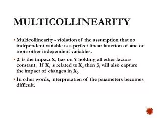
Chapter 10 Multicollinearity 2 Chapter Introduction One of the assumption of the classical linear regression model (CLRM) is that there is no multicollinearity among the independent variables included in the regression model. In this chapter we take a critical look at this assumption by seeking answers to the following questions: 1. What is the nature of multicollinearity? 2. Is multicollinearity really a problem? 3. What are its practical consequences? 4. How does one detect it? 5. What remedial measures can be taken to alleviate the problem of multicollinear- ity? In this chapter we also discuss Assumption 6 of the CLRM, namely, that the number of observations in the sample must be greater than the number of regressors, and Assumption 7, which requires that there be sufficient variability in the values of the regressors, for they are intimately related to the assumption of no multicollinearity. Book: Basic Econometrics 5thEdition Written by: Damodar N. Gujarati Dawn C. Porter Muhammad Ali, PhD Scholar (Department of Statistics Abdul Wali Khan University, Mardan, Pakistan.) Chapter 10 : Multicollinearity 2 / 43
Chapter 10 Multicollinearity 3 10.1 Nature of Multicollinearity The term multicollinearity was introduced by Ragnar Frisch, meaning that there is perfect linear relationship among some or all explanatory variables. k-variable regression involving explanatory variables X1,X2,...,Xk an exact linear relationship is said to exist if the following condition is satisfied: For the λ1X1+ λ2X2+ ... + λkXk= 0 (10.1) where λ1,λ2, ... , λkare constants such that not all of them are zero simultaneously, equation 1 shows that there is perfect multicollinearity between the regressors. The relationship between independent variables may not always be perfect, there are cases when the independent variables may be correlated but not perfectly. This relationship between regressors can be seen as follows: λ1X1+ λ2X2+ ... + λkXk+ ?i= 0 (10.2) where ?iis a stochastic error term. Book: Basic Econometrics 5thEdition Written by: Damodar N. Gujarati Dawn C. Porter Muhammad Ali, PhD Scholar (Department of Statistics Abdul Wali Khan University, Mardan, Pakistan.) Chapter 10 : Multicollinearity 3 / 43
Chapter 10 Multicollinearity 4 To see the difference between perfect and less than perfect multicollinearity, assume, for example, that λ26= 0. Then, Eq. (10.1) can be written as: X2i= −λ1 λ2X1−λ3 λ2X3− ... −λk (10.3) λ2Xki which shows how X2is exactly linearly related to other variables. In this situation, the coefficient of correlation between the variable X2and the linear combination on the right side of Eq. (10.3) is 1. Similarly, if λ26= 0, Eq. (10.2) can be written as: 1 X2i= −λ1 λ2X1−λ3 λ2X3− ... −λk (10.4) λ2Xki− λ2?i which shows that X2is not an exact linear combination of other X’s because it is also determined by the stochastic error term ?i. Book: Basic Econometrics 5thEdition Written by: Damodar N. Gujarati Dawn C. Porter Muhammad Ali, PhD Scholar (Department of Statistics Abdul Wali Khan University, Mardan, Pakistan.) Chapter 10 : Multicollinearity 4 / 43
Chapter 10 Multicollinearity 5 Numerical Example As a numerical example, consider the following hypothetical data: Table 1: Hypothetical Data X2 10 15 18 24 30 X3 50 75 90 120 150 X4 52 75 97 129 152 It can be seen that X3i= 5X2i. Therefore, there is perfect collinearity between X2 and X3since the coefficient of correlation r23is 1. The variable X4was created from X3by simply adding to it the following numbers, which were taken from a table of random numbers: 2, 0, 7, 9, 2. Now there is no longer perfect collinearity between X2and X4. However, the two variables are highly correlated because calculations will show that the coefficient of correlation between them is 0.9959. Book: Basic Econometrics 5thEdition Written by: Damodar N. Gujarati Dawn C. Porter Muhammad Ali, PhD Scholar (Department of Statistics Abdul Wali Khan University, Mardan, Pakistan.) Chapter 10 : Multicollinearity 5 / 43
Chapter 10 Multicollinearity 6 Algebraic approach to multicollinearity Multicollinearity can be portrayed by the Ballentine presented in Figure 1. In this figure the circles Y, X2, and X3represent, respectively, the variations in Y and X2 and X3. The degree of collinearity can be measured by the extent of the overlap (shaded area) of the X2and X3circles. In Figure 10.1a there is no overlap between X2and X3, and hence no collinearity. In Figure 1b through 1e there is a “low” to “high” degree of collinearity—the greater the overlap between X2and X3the higher the degree of collinearity. Figure 1: The Ballentine view of multicollinearity Muhammad Ali, PhD Scholar (Department of Statistics Abdul Wali Khan University, Mardan, Pakistan.) Book: Basic Econometrics 5thEdition Written by: Damodar N. Gujarati Dawn C. Porter Chapter 10 : Multicollinearity 6 / 43
Chapter 10 Multicollinearity 7 Technical Note Note that multicollinearity refers only to linear relationships among the X variables. It does not rule out nonlinear relationships among them. For example, consider the following regression model: Yi= β0+ β1Xi+ β2X2 i+ β3X3 (10.5) i+ ?i where, say, Y = total cost of production and X = output. The variables Xi2(output squared) and Xi3(output cubed) are obviously functionally related to Xi , but the relationship is nonlinear. Strictly, therefore, models such as Eq. (10.5) do not violate the assumption of no multicollinearity. If multicollinearity is perfect in the sense of Eq.(10.1), the regression coefficients of the X variables are indeterminate and their standard errors are infinite. If mul- ticollinearity is less than perfect, as in Eq. (10.2), the regression coefficients, al- though determinate, possess large standard errors (in relation to the coefficients themselves), which means the coefficients cannot be estimated with great precision or accuracy. Book: Basic Econometrics 5thEdition Written by: Damodar N. Gujarati Dawn C. Porter Muhammad Ali, PhD Scholar (Department of Statistics Abdul Wali Khan University, Mardan, Pakistan.) Chapter 10 : Multicollinearity 7 / 43
Chapter 10 Multicollinearity 8 Why does the classical linear regression model assume that there is no multicollinear- ity among the X’s? The reasoning is this: If multicollinearity is perfect in the sense of Eq. (10.1), the regression coefficients of the X variables are indeterminate and their standard errors are infinite. If multicollinearity is less than perfect, as in Eq. (10.2), the regression coefficients, although determinate, possess large standard er- rors (in relation to the coefficients themselves), which means the coefficients cannot be estimated with great precision or accuracy. Reasons of Multicollinearity 1. The data collection method employed: For example, sampling over a limited range of the values taken by the regressors in the population. 2. Constraints on the model or in the population being sampled: For example, in the regression of electricity consumption on income (X2) and house size (X3) there is a physical constraint in the population in that families with higher incomes generally have larger homes than families with lower incomes. 3. Model specification: For example, adding polynomial terms to a regression model, especially when the range of the X variable is small. 4. An over-determined model: This happens when the model has more explanatory variables than the number of observations. This could happen in medical research. Book: Basic Econometrics 5thEdition Written by: Damodar N. Gujarati Dawn C. Porter Muhammad Ali, PhD Scholar (Department of Statistics Abdul Wali Khan University, Mardan, Pakistan.) Chapter 10 : Multicollinearity 8 / 43
Chapter 10 Multicollinearity 9 An additional reason for multicollinearity, especially in time series data, may be that the regressors included in the model share a common trend, that is, they all increase or decrease over time. 10.2 Estimation in the Presence of Perfect Multicollinearity It was stated previously that in the case of perfect multicollinearity the regression coefficients remain indeterminate and their standard errors are infinite. Using the deviation form, where all the variables are expressed as deviations from their sample means, we can write the three-variable regression model as: yi=ˆβ2x2i+ˆβ3x3i+ ˆ ?i (10.6) we know that ˆβ2=(Pyix2i)(Px32 ˆβ3=(Pyix3i)(Px22 i) − (Pyix3i)(Px2ix3i) i) − (Pyix2i)(Px2ix3i) (10.7) (Px22 (Px22 Chapter 10 : Multicollinearity i)(Px32 i)(Px32 i) − (Px2ix3i)2 i) − (Px2ix3i)2 (10.8) Book: Basic Econometrics 5thEdition Written by: Damodar N. Gujarati Dawn C. Porter Muhammad Ali, PhD Scholar (Department of Statistics Abdul Wali Khan University, Mardan, Pakistan.) 9 / 43
Chapter 10 Multicollinearity 10 Assume that X3i= λX2i, where λ is a nonzero constant (e.g., 2, 4, 1.8, etc.). Substituting this into Eq. (10.7), we obtain ˆβ2=(Pyix2i)(λ2Px22 ˆβ2=λ2(Pyix2i)(Px22 =0 i) − (λPyix2i)(λPx22 i) − λ2(Pyix2i)(Px22 i) (10.9) (Px22 i)(λ2Px22 λ2(Px22 i) − λ2(Px22 i)2− λ2(Px22 0 i)2 i) (10.10) i)2 which is an indeterminate expression (verify thatˆβ3is also indeterminate). 10.3 Estimation in the Presence of “High” but “Imperfect” Multicollinearity The perfect multicollinearity situation is a pathological extreme. Generally, there is no exact linear relationship among the X variables, especially in data involving economic time series. Thus, turning to the three-variable model in the deviation form given in Eq. (10.6), instead of exact multicollinearity, we may have Book: Basic Econometrics 5thEdition Written by: Damodar N. Gujarati Dawn C. Porter Muhammad Ali, PhD Scholar (Department of Statistics Abdul Wali Khan University, Mardan, Pakistan.) Chapter 10 : Multicollinearity 10 / 43
Chapter 10 Multicollinearity 11 (10.11) x3i= λx2i+ ?i where λ 6= 0 and where ?i is a stochastic error term such thatPx2i?i = 0. The case, estimation of regression coefficients β2and β3may be possible. For example, substituting Eq. (10.11) into Eq. (10.7), we obtain Ballentines shown in Figure 1b to 1e represent cases of imperfect collinearity. In this ˆβ2=(Pyix2i)(λ2Px22 where use is made ofPx2i?i = 0. A similar expression can be derived forˆβ3. estimated. Of course, if ?iis sufficiently small, say, very close to zero, Eq. (10.11) will indicate almost perfect collinearity and we shall be back to the indeterminate case of Eq. (10.10). i+P?2 i) − (λPyix2i+Pyi?i)(λPx22 i) (10.12) Px22 i(λ2Px22 i+P?2 i) − (λPx22 i)2 Now, unlike Eq. (10.10), there is no reason to believe that Eq. (10.12) cannot be Book: Basic Econometrics 5thEdition Written by: Damodar N. Gujarati Dawn C. Porter Muhammad Ali, PhD Scholar (Department of Statistics Abdul Wali Khan University, Mardan, Pakistan.) Chapter 10 : Multicollinearity 11 / 43
Chapter 10 Multicollinearity 12 10.4 Theoretical Consequences of Multicollinearity Recall that if the assumptions of the classical model are satisfied, the OLS esti- mators of the regression estimators are BLUE. Now it can be shown that even if multicollinearity is very high, as in the case of near multicollinearity, the OLS estimators still retain the property of BLUE. As Christopher Achen remarks Beginning students of methodology occasionally worry that their independent variables are correlated—the so-called multicollinearity problem. But multicollinearity violates no regression assumptions. Unbiased, con- sistent estimates will occur, and their standard errors will be correctly estimated. The only effect of multicollinearity is to make it hard to get coefficient estimates with small standard error. First, it is true that even in the case of near multicollinearity the OLS estimators are unbiased. But unbiasedness is a multisample or repeated sampling property. What it means is that, keeping the values of the X variables fixed, if one obtains repeated samples and computes the OLS estimators for each of these samples, the average of the sample values will converge to the true population values of the estimators as the number of samples increases. But this says nothing about the properties of estimators in any given sample. Muhammad Ali, PhD Scholar (Department of Statistics Abdul Wali Khan University, Mardan, Pakistan.) Chapter 10 : Multicollinearity Book: Basic Econometrics 5thEdition Written by: Damodar N. Gujarati Dawn C. Porter 12 / 43
Chapter 10 Multicollinearity 13 Second, it is also true that collinearity does not destroy the property of minimum variance: In the class of all linear unbiased estimators, the OLS estimators have minimum variance; that is, they are efficient. But this does not mean that the variance of an OLS estimator will necessarily be small (in relation to the value of the estimator) in any given sample, as we shall demonstrate shortly. Third, multicollinearity is essentially a sample (regression) phenomenon in the sense that, even if the X variables are not linearly related in the population, they may be so related in the particular sample at hand: When we consider the population regression function (PRF), we believe that all the X variables included in the model have a separate or independent influence on the dependent variable Y. But it may happen that in any given sample that is used to test the PRF some or all of the X variables are so highly collinear that we cannot isolate their individual influence on Y. So to speak, our sample lets us down, although the theory says that all the X’s are important. In short, our sample may not be “rich” enough to accommodate all X variables in the analysis. Book: Basic Econometrics 5thEdition Written by: Damodar N. Gujarati Dawn C. Porter Muhammad Ali, PhD Scholar (Department of Statistics Abdul Wali Khan University, Mardan, Pakistan.) Chapter 10 : Multicollinearity 13 / 43
Chapter 10 Multicollinearity 14 As an illustration, reconsider the consumption–income example of Chapter 3 (Ex- ample 3.1): Consumption = β1+ β2Income + β3Wealth + ui Now it may happen that when we obtain data on income and wealth, the two variables may be highly correlated: Wealthier people generally tend to have higher incomes. Thus, although in theory income and wealth are logical candidates to explain the behavior of consumption expenditure, in practice (i.e., in the sample) it may be difficult to disentangle the separate influences of income and wealth on consumption expenditure. 10.5 Practical Consequences of Multicollinearity In cases of near or high multicollinearity, one is likely to encounter the following consequences: 1. Although BLUE, the OLS estimators have large variances and covariances, making precise estimation difficult. 2. Because of consequence 1, the confidence intervals tend to be much wider, leading to the acceptance of the “zero null hypothesis”. Book: Basic Econometrics 5thEdition Written by: Damodar N. Gujarati Dawn C. Porter Muhammad Ali, PhD Scholar (Department of Statistics Abdul Wali Khan University, Mardan, Pakistan.) Chapter 10 : Multicollinearity 14 / 43
Chapter 10 Multicollinearity 15 3. Also because of consequence 1, the t ratio of one or more coefficients tends to be statistically insignificant. 4. Although the t ratio of one or more coefficients is statistically insignificant, R2 , the overall measure of goodness of fit, can be very high. 5. The OLS estimators and their standard errors can be sensitive to small changes in the data. The preceding consequences can be demonstrated as follows. Large Variances and Covariances of OLS Estimators To see large variances and covariances, recall that for the model (6) the variances and covariances ofˆβ2andˆβ3are given by σ2 i(1 − r22 σ2 i(1 − r22 −r23σ2 var(ˆβ2) = (10.12) Px22 Px32 (1 − r22 3) var(ˆβ3) = (10.13) 3) cov(ˆβ2,ˆβ3) = (10.14) 3)pPx22 Px32 i i Book: Basic Econometrics 5thEdition Written by: Damodar N. Gujarati Dawn C. Porter Muhammad Ali, PhD Scholar (Department of Statistics Abdul Wali Khan University, Mardan, Pakistan.) Chapter 10 : Multicollinearity 15 / 43
Chapter 10 Multicollinearity 16 where r23is the coefficient of correlation between X2and X3. It is apparent from Eqs. (10.13) and (10.14) that as r23tends toward 1, that is, as collinearity increases, the variances of the two estimators increase and in the limit when r23= 1, they are infinite. It is equally clear from Eq. (10.15) that as r23increases toward 1, the covariance of the two estimators also increases in absolute value. The speed with which variances and covariances increase can be seen with the variance-inflating factor (VIF), which is defined as 1 (10.15) VIF = (1 − r22 3) VIF shows how the variance of an estimator is inflated by the presence of multi- collinearity. As r23approaches 1, the VIF approaches infinity. That is, as the extent of collinearity increases, the variance of an estimator increases, and in the limit it can become infinite. As can be readily seen, if there is no collinearity between X2and X3, VIF will be 1. Using this definition, we can express Eqs. (10.13) and (10.14) as Book: Basic Econometrics 5thEdition Written by: Damodar N. Gujarati Dawn C. Porter Muhammad Ali, PhD Scholar (Department of Statistics Abdul Wali Khan University, Mardan, Pakistan.) Chapter 10 : Multicollinearity 16 / 43
Chapter 10 Multicollinearity 17 σ2 (10.16) Px22 Px32 var(β2) = VIF i σ2 (10.17) var(β3) = VIF i To give some idea about how fast the variances and covariances increase as r23 increases, consider Table 1, which gives these variances and covariances for selected values of r23. As this table shows, increases in r23have a dramatic effect on the estimated variances and covariances of the OLS estimators. When r23= 0.50, the var(2) is 1.33 times the variance when r23is zero, but by the time r23reaches 0.95 it is about 10 times as high as when there is no collinearity. An increase of r23 from 0.95 to 0.995 makes the estimated variance 100 times that when collinearity is zero. The same dramatic effect is seen on the estimated covariance. All this can be seen in Figure 2. Book: Basic Econometrics 5thEdition Written by: Damodar N. Gujarati Dawn C. Porter Muhammad Ali, PhD Scholar (Department of Statistics Abdul Wali Khan University, Mardan, Pakistan.) Chapter 10 : Multicollinearity 17 / 43
Chapter 10 Multicollinearity 18 Table 2: The Effect of Increasing r23 on var(ˆβ2) and cov(ˆβ2,ˆβ3) var(ˆβ2)(r236=0) var(ˆ β2)(r23=0) (4) - 1.33 1.96 2.78 5.26 10.26 16.92 50.25 100.00 500.00 var(ˆβ2) (3) σ2 Σx22 i 1.33×A 1.96×A 2.78×A 5.26×A 10.26×A 16.92×A 50.25×A 100.00×A 500.00×A Note: B= cov(ˆβ2,ˆβ3) (5) 0 0.67×B 1.37×B 2.22×B 4.73×B 9.74×B 16.41×B 49.75×B 99.50×B 499.50×B Values of r23 (1) 0.00 0.50 0.70 0.80 0.90 0.95 0.97 0.99 0.995 0.999 VIF (2) 1.00 1.33 1.96 2.78 5.76 10.26 16.92 50.25 100.00 500.00 = A −σ2 Σx22 √ iΣx32 i Book: Basic Econometrics 5thEdition Written by: Damodar N. Gujarati Dawn C. Porter Muhammad Ali, PhD Scholar (Department of Statistics Abdul Wali Khan University, Mardan, Pakistan.) Chapter 10 : Multicollinearity 18 / 43
Chapter 10 Multicollinearity 19 Before proceeding further, it may be noted that the inverse of the VIF is called tolerance (TOL). That is, 1 = (1 − R2 (10.18) TOLj= j) VIFj When R2 collinearity whatsoever), TOLj is 1. Because of the intimate connection between VIF and TOL, one can use them interchangeably. Wider Confidence Intervals Because of the large standard errors, the confidence intervals for the relevant popu- lation parameters tend to be larger, as can be seen from Table 3. For example, when r23= 0.95, the confidence interval for β2is larger than when r23= 0 by a factor of data may be compatible with a diverse set of hypotheses. Hence, the probability of accepting a false hypothesis (i.e., type II error) increases. j= 1 (i.e., perfect collinearity), TOLj = 0 and when R2 j= 0 (i.e., no √10.26, or about 3. Therefore, in cases of high multicollinearity, the sample Book: Basic Econometrics 5thEdition Written by: Damodar N. Gujarati Dawn C. Porter Muhammad Ali, PhD Scholar (Department of Statistics Abdul Wali Khan University, Mardan, Pakistan.) Chapter 10 : Multicollinearity 19 / 43
Chapter 10 Multicollinearity 20 Table 3: The Effect of Increasing Collinearity on the 95% Confidence Interval for β2 Values of r23 0.00 95% Confidence Interval for β2 ˆβ2± 1.96 ˆβ2± 1.96p(1.33) ˆβ2± 1.96p(100) q σ2 q q Px22 q q i σ2 0.50 Px22 Px22 Px22 Px22 ˆβ2± 1.96p(10.26) ˆβ2± 1.96p(500) i σ2 0.95 i σ2 0.995 i σ2 0.999 i “Insignificant” t Ratios Recall that to test the null hypothesis that, say, β2= 0, we use the t ratio, that is,ˆβ2/se(ˆβ2) and compare the estimated t value with the critical t value from the t table. But as we have seen, in cases of high collinearity the estimated standard errors increase dramatically, thereby making the t values smaller. Therefore, in such cases, the null hypothesis is accepted. Book: Basic Econometrics 5thEdition Written by: Damodar N. Gujarati Dawn C. Porter Muhammad Ali, PhD Scholar (Department of Statistics Abdul Wali Khan University, Mardan, Pakistan.) Chapter 10 : Multicollinearity 20 / 43
Chapter 10 Multicollinearity 21 A High R2but Few Significant t Ratios Consider the k-variable linear regression model: Yi= β1+ β2X2i+ β3X3i+ ... + βkXki+ ui In cases of high collinearity, it is possible to find, as we have just noted, that one or more of the partial slope coefficients are individually statistically insignificant on the basis of the t test. Yet the R2in such situations may be so high, say, in excess of 0.9, that on the basis of the F test one can convincingly reject the hypothesis that β2= β3= ···= βk= 0. Sensitivity of OLS Estimators and Their Standard Errors to Small Changes in Data As long as multicollinearity is not perfect, estimation of the regression coefficients is possible but the estimates and their standard errors become very sensitive to even the slightest change in the data. Book: Basic Econometrics 5thEdition Written by: Damodar N. Gujarati Dawn C. Porter Muhammad Ali, PhD Scholar (Department of Statistics Abdul Wali Khan University, Mardan, Pakistan.) Chapter 10 : Multicollinearity 21 / 43
Chapter 10 Multicollinearity 22 To see this, consider Table 4. Based on these data, we obtain the following multiple regression: ˆYi= 1.1939 + 0.4463X2i+ 0.0030X3i SE = (0.7737) (0.1848) (0.0851) t = (1.5431) (2.4151) (0.0358) R2= 0.8101 r23= 0.5523 cov(ˆβ2,ˆβ3) = −0.00868 ,df = 2 Regression (20) shows that none of the regression coefficients is individually sig- nificant at the conventional 1 or 5 percent levels of significance, althoughˆβ2 is significant at the 10 percent level on the basis of a one-tail t test. Now consider Table 5. The only difference between Tables 4 and 5 is that the third and fourth values of X3are interchanged. Using the data of Table 5, we now obtain (10.19) Book: Basic Econometrics 5thEdition Written by: Damodar N. Gujarati Dawn C. Porter Muhammad Ali, PhD Scholar (Department of Statistics Abdul Wali Khan University, Mardan, Pakistan.) Chapter 10 : Multicollinearity 22 / 43
Chapter 2 Multicollinearity 23 ˆYi= 1.2108 + 0.4014X2i+ 0.0270X3i SE = (0.7480) (0.2721) (0.1252) t = (1.6197) (1.4752) (0.2158) R2= 0.8143 r23= 0.8285 cov(ˆβ2,ˆβ3) = −0.0282 ,df = 2 As a result of a slight change in the data, we see thatˆβ2, which was statistically significant before at the 10 percent level of significance, is no longer significant even at that level. Also note that in Eq. (10.19) cov (ˆβ2,ˆβ3)= −0.00868 whereas in Eq. (10.20) it is −0.0282, a more than threefold increase. All these changes may be attributable to increased multicollinearity: In Eq. (10.19) r23= 0.5523, whereas in Eq. (10.20) it is 0.8285. Similarly,standard errors ofˆβ2andˆβ3increase between the two regressions, a usual symptom of collinearity. (10.20) Book: Basic Econometrics 5thEdition Written by: Damodar N. Gujarati Dawn C. Porter Muhammad Ali, PhD Scholar (Department of Statistics Abdul Wali Khan University, Mardan, Pakistan.) Chapter 10 : Multicollinearity 23 / 43
Chapter 2 Multicollinearity 24 Table 4: Hypothetical Data on Y,X2 and X3 Table 5: Hypothetical Data on Y,X2 and X3 Y 1 2 3 4 5 Y 1 2 3 4 5 X2 2 0 4 6 8 X3 4 2 12 0 16 X2 2 0 4 6 8 X3 4 2 0 12 16 We noted earlier that in the presence of high collinearity one cannot estimate the individual regression coefficients precisely but that linear combinations of these coefficients may be estimated more precisely. This fact can be substantiated from the regressions (10.19) and (10.20). In the first regression the sum of the two partial slope coefficients is 0.4493 and in the second it is 0.4284, practically the same. Not only that, their standard errors are practically the same, 0.1550 vs. 0.1823.14. Note, however, the coefficient of X3 has changed dramatically, from 0.003 to 0.027. Book: Basic Econometrics 5thEdition Written by: Damodar N. Gujarati Dawn C. Porter Muhammad Ali, PhD Scholar (Department of Statistics Abdul Wali Khan University, Mardan, Pakistan.) Chapter 10 : Multicollinearity 24 / 43
Chapter 2 Multicollinearity 25 10.6 An Illustrative Example Example 10.1 Consumption Expenditure in Relation to Income and Wealth To illustrate the various points made thus far, let us consider the consump- tion–income example from the introduction. Table 6 contains hypothetical data on consumption, income, and wealth. If we assume that consumption expenditure is linearly related to income and wealth, then, from Table 6 we obtain the following regression: ˆYi= 24.7747 + 0.9415X2i− 0.0424X3i SE = (6.7525) (0.8229) (0.0807) t = (3.6690) (1.1442) (−0.5261) R2= 0.9635, ¯R2= 0.9531, (10.21) df = 7 Book: Basic Econometrics 5thEdition Written by: Damodar N. Gujarati Dawn C. Porter Muhammad Ali, PhD Scholar (Department of Statistics Abdul Wali Khan University, Mardan, Pakistan.) Chapter 10 : Multicollinearity 25 / 43
Chapter 10 Multicollinearity 26 Example 10.6 (Continued) Table 6: Hypothetical Data on Consumption Expenditure Y, Income X2,and Wealth X3 Y$ 70 65 90 95 110 115 120 140 155 150 X3,$ 80 100 120 140 160 180 200 220 240 260 X4$ 810 1009 1273 1425 1633 1876 2052 2201 2435 2686 Book: Basic Econometrics 5thEdition Written by: Damodar N. Gujarati Dawn C. Porter Muhammad Ali, PhD Scholar (Department of Statistics Abdul Wali Khan University, Mardan, Pakistan.) Chapter 10 : Multicollinearity 26 / 43
Chapter 10 Multicollinearity 27 Example 10.6 (Continued) Table 7: ANOVA Table for the Consumption– Income–Wealth Example Source of Variation Due to regression Due to residual SS df 2 7 MSS 8,565.5541 324.4459 4,282.7770 46.3494 Regression (10.21) shows that income and wealth together explain about 96 percent of the variation in consumption expenditure, and yet neither of the slope coefficients is individually statistically significant. Moreover, not only is the wealth variable statistically insignificant but also it has the wrong sign. A priori, one would expect a positive relationship between consumption and wealth. Althoughˆβ2andˆβ3are individually statistically insignificant, if we test the hypothesis that β2= β3= 0 simultaneously, this hypothesis can be rejected, as Table 7 shows. Under the usual assumption we obtain F =4282.7770 46.3494 = 92.4019 (10.22) Book: Basic Econometrics 5thEdition Written by: Damodar N. Gujarati Dawn C. Porter Muhammad Ali, PhD Scholar (Department of Statistics Abdul Wali Khan University, Mardan, Pakistan.) Chapter 10 : Multicollinearity 27 / 43
Chapter 10 Multicollinearity 28 Example 10.6 (Continued) This F value is obviously highly significant. It is interesting to look at this result geometrically. (See Figure 2). Figure 2: Individual confidence intervals for β2 and β3 and joint confidence interval (ellipse) for 2 and 3. Based on the regression (10.21), we have established the individual 95 percent confidence intervals for β2and β3following the usual procedure discussed in Chapter 8. As these intervals show, individually each of them includes the value of zero. Therefore, individually we can accept the hypothesis that the two partial slopes are zero. But, when we establish the joint confidence interval to test (Continued) Book: Basic Econometrics 5thEdition Written by: Damodar N. Gujarati Dawn C. Porter Muhammad Ali, PhD Scholar (Department of Statistics Abdul Wali Khan University, Mardan, Pakistan.) Chapter 10 : Multicollinearity 28 / 43
Chapter 10 Multicollinearity 29 Example 10.6 (Continued) the hypothesis that β2 = β3 = 0, that hypothesis cannot be accepted since the joint confidence interval, actually an ellipse, does not include the origin. As already pointed out, when collinearity is high, tests on individual regressors are not reliable; in such cases it is the overall F test that will show if Y is related to the various regressors. Our example shows dramatically what multicollinearity does. The fact that the F test is significant but the t values of X2and X3are individually insignif- icant means that the two variables are so highly correlated that it is impossible to isolate the individual impact of either income or wealth on consumption. As a matter of fact, if we regress X3on X2, we obtain ˆ X3i= 7.5454 + 10.1909X2i SE = (29.4758) (0.1643) t = (0.2560) (62.0405) R2= 0.99979 (10.23) Book: Basic Econometrics 5thEdition Written by: Damodar N. Gujarati Dawn C. Porter Muhammad Ali, PhD Scholar (Department of Statistics Abdul Wali Khan University, Mardan, Pakistan.) Chapter 10 : Multicollinearity 29 / 43
Chapter 10 Multicollinearity 30 Example 10.6 (Continued) which shows that there is almost perfect collinearity between X3and X2. Now let us see what happens if we regress Y on X2only: ˆYi= 24.4545 + 0.5091X2i SE = (6.4138) (0.0357) t = (3.8128) (14.2432) R2= 0.9621 (10.24) In Eq. (10.21) the income variable was statistically insignificant, whereas now it is highly significant. If instead of regressing Y on X2, we regress it on X3, we obtain ˆYi= 24.411 + 0.0498X3i SE = (6.874) (0.0037) t = (3.551) (13.29) R2= 0.9567 (10.25) Book: Basic Econometrics 5thEdition Written by: Damodar N. Gujarati Dawn C. Porter Muhammad Ali, PhD Scholar (Department of Statistics Abdul Wali Khan University, Mardan, Pakistan.) Chapter 10 : Multicollinearity 30 / 43
Chapter 10 Multicollinearity 31 Example 10.6 (Continued) We see that wealth has now a significant impact on consumption expenditure, whereas in Eq. (10.21) it had no effect on consumption expenditure. Regressions (10.24) and (10.25) show very clearly that in situations of extreme multicollinearity dropping the highly collinear variable will often make the other X variable statistically significant. This result would suggest that a way out of extreme collinearity is to drop the collinear variable, but we shall have more to say about it in Section 10.8. 10.7 Detection of Multicollinearity Since multicollinearity is essentially a sample phenomenon, arising out of the largely nonexperimental data collected in most social sciences, we do not have one unique method of detecting it or measuring its strength. What we have are some rules of thumb, some informal and some formal, but rules of thumb all the same. We now consider some of these rules. 1. High R2but few significant t ratios. As noted, this is the “classic” symptom of multicollinearity. If R2is high, say, in excess of 0.8, the F test in most cases will reject the hypothesis that the partial slope coefficients are simultaneously equal to zero, but the individual t tests will show that none or very few of the partial slope coefficients are statistically different from zero. Muhammad Ali, PhD Scholar (Department of Statistics Abdul Wali Khan University, Mardan, Pakistan.) Chapter 10 : Multicollinearity Book: Basic Econometrics 5thEdition Written by: Damodar N. Gujarati Dawn C. Porter 31 / 43
Chapter 10 Multicollinearity 32 2. High pair-wise correlations among regressors. Another suggested rule of thumb is that if the pair-wise or zero-order correlation coefficient between two regressors is high, say, in excess of 0.8, then multicollinearity is a serious problem. To put the matter somewhat technically, high zero-order correlations are a sufficient but not a necessary condition for the existence of multicollinearity because it can exist even though the zero-order or simple correlations are comparatively low (say, less than 0.50). To see this relationship, suppose we have a four-variable model: (10.26) Yi= β1+ β2X2i+ β3X3i+ β4X4i+ ui and suppose that (10.27) X4i= λ2X2i+ λ3X3i where λ2 and λ3 are constants, not both zero. Obviously, X4 is an exact linear combination of X2and X3, giving R2 regression of X4on X2and X3. Now recalling the formula (7.11.5) from Chapter 7, we can write Muhammad Ali, PhD Scholar (Department of Statistics Abdul Wali Khan University, Mardan, Pakistan.) Chapter 10 : Multicollinearity 4.32= 1, the coefficient of determination in the Book: Basic Econometrics 5thEdition Written by: Damodar N. Gujarati Dawn C. Porter 32 / 43
Chapter 10 Multicollinearity 33 4.23=r2 42+ r2 43− 2r42r43r23 1 − r2 R2 (10.28) 23 But since R2 4.23= 1 because of perfect collinearity, we obtain 1 =r2 42+ r2 43− 2r42r43r23 1 − r2 (10.29) 23 Eq. (10.28) is satisfied by r42= 0.5, r43= 0.5, and r23= 0.5, which are not very high values. Therefore, in models involving more than two explanatory variables, the simple or zero order correlation will not provide an infallible guide to the presence of multicollinearity. Of course, if there are only two explanatory variables, the zero- order correlations will suffice. 3. Examination of partial correlations. It is suggested that one should look at the partial correlation coefficients. Thus, in the regression of Y on X2, X3, and X4, a finding that R2 low may suggest that the variables X2, X3, and X4are highly inter-correlated and that at least one of these variables is unnecessary. 1.234is very high but r2 12.34, r2 13.24, and r2 14.23are comparatively Book: Basic Econometrics 5thEdition Written by: Damodar N. Gujarati Dawn C. Porter Muhammad Ali, PhD Scholar (Department of Statistics Abdul Wali Khan University, Mardan, Pakistan.) Chapter 10 : Multicollinearity 33 / 43
Chapter 10 Multicollinearity 34 4. Auxiliary regressions. Since multicollinearity arises because one or more of the regressors are exact or approximately linear combinations of the other regressors, one way of finding out which X variable is related to other X variables is to regress each Xi on the remaining X variables and compute the corresponding R2, which we designate as R2 auxiliary to the main regression of Y on the X’s. Then, following the relationship between F and R2established i; each one of these regressions is called an auxiliary regression, R2 xi.x2x3...xk/(k − 2) (1 − R2 (10.30) Fi= xi.x2x3...xk)/(n − k + 1) Fi follows the F distribution with k - 2 and n - k + 1 df. In Eq. (10.30) n stands for the sample size, k stands for the number of explanatory variables including the intercept term, and R2 of variable Xion the remaining X variables. If the computed F exceeds the critical Fi at the chosen level of significance, it is taken to mean that the particular Xi is collinear with other X’s; if it does not exceed the critical Fi, we say that it is not collinear with other X’s, in which case we may retain that variable in the model. xi.x2x3...xkis the coefficient of determination in the regression Book: Basic Econometrics 5thEdition Written by: Damodar N. Gujarati Dawn C. Porter Muhammad Ali, PhD Scholar (Department of Statistics Abdul Wali Khan University, Mardan, Pakistan.) Chapter 10 : Multicollinearity 34 / 43
Chapter 10 Multicollinearity 35 5. Eigenvalues and condition index. we can find the eigenvalues and the condi- tion index(usually with the help of any software like EViews, SAS, Stata, R etc) to diagnose multicollinearity. From these eigenvalues, however, we can derive what is known as the condition number k defined as k =Maximum eigenvalue Minimum eigenvalue and the condition index (CI) defined as s √ Maximum eigenvalue Minimum eigenvalue= CI = k Then we have this rule of thumb: If k is between 100 and 1000 there is moderate to strong multicollinearity and if it exceeds 1000 there is severe multicollinearity. Alternatively, if the CI ( = multicollinearity and if it exceeds 30 there is severe multicollinearity. √k) is between 10 and 30, there is moderate to strong Book: Basic Econometrics 5thEdition Written by: Damodar N. Gujarati Dawn C. Porter Muhammad Ali, PhD Scholar (Department of Statistics Abdul Wali Khan University, Mardan, Pakistan.) Chapter 10 : Multicollinearity 35 / 43
Chapter 10 Multicollinearity 36 6. Tolerance and variance inflation factor We have already introduced TOL and VIF. As R2 in the regression of regressor Xjon the remaining regressors in the model, increases toward unity, that is, as the collinearity of Xj with the other regressors increases, VIF also increases and in the limit it can be infinite. Some authors therefore use the VIF as an indicator of multicollinearity. The larger the value of VIFj, the more “troublesome” or collinear the variable Xj. As a rule of thumb, if the VIF of a variable exceeds 10, which will happen if R2 highly collinear. Of course, one could use TOLjas a measure of multicollinearity in view of its intimate connection with VIFj. The closer TOLj is to zero, the greater the degree of collinearity of that variable with the other regressors. On the other hand, the closer TOLjis to 1, the greater the evidence that Xjis not collinear with the other regressors. j, the coefficient of determination jexceeds 0.90, that variable is said be Book: Basic Econometrics 5thEdition Written by: Damodar N. Gujarati Dawn C. Porter Muhammad Ali, PhD Scholar (Department of Statistics Abdul Wali Khan University, Mardan, Pakistan.) Chapter 10 : Multicollinearity 36 / 43
Chapter 10 Multicollinearity 37 10.8 Remedial Measures Rule-of-Thumb Procedures Following are the some of rule of thumb procedures to address the problem of multicollinearity; their success will depend on the severity of the collinearity problem. 1. A priori information. Suppose we consider the following model Yi= β1+ β2X2i+ β3X3i+ ui where Y = consumption, X2= income, and X3= wealth. As noted before, income and wealth variables tend to be highly collinear. Suppose that β3= 0.10β2; that is, the rate of change of consumption with respect to wealth is one-tenth the cor- responding rate with respect to income. We can then run the following regression: Yi= β1+ β2X2i+ 0.10β2X3i+ ui = β1+ β2Xi+ ui Once we obtainˆβ2 we can estimateˆβ3 from the where Xi = X2i + 0.1X3i. postulated relationship between β2and β3. Book: Basic Econometrics 5thEdition Written by: Damodar N. Gujarati Dawn C. Porter Muhammad Ali, PhD Scholar (Department of Statistics Abdul Wali Khan University, Mardan, Pakistan.) Chapter 10 : Multicollinearity 37 / 43
Chapter 10 Multicollinearity 38 2. Combining cross-sectional and time series data. A variant of the extraneous or a priori information technique is the combination of cross-sectional and time series data, known as pooling the data. Suppose we want to study the demand for automobiles in the United States and assume we have time series data on the number of cars sold, average price of the car, and consumer income. Suppose also that ln Yt= β1+ β2lnPt+ β3lnIt+ ut where Y = number of cars sold, P = average price, I = income, and t = time. Our objective is to estimate the price elasticity, β2, and income elasticity, β3. In time series data the price and income variables generally tend to be highly collinear. Therefore, if we run the preceding regression, we shall be faced with the usual multicollinearity problem. Let the cross-sectionally estimated income elasticity be ˆβ3. Using this estimate, we may write the above time series regression as Book: Basic Econometrics 5thEdition Written by: Damodar N. Gujarati Dawn C. Porter Muhammad Ali, PhD Scholar (Department of Statistics Abdul Wali Khan University, Mardan, Pakistan.) Chapter 10 : Multicollinearity 38 / 43
Chapter 10 Multicollinearity 39 ln Yt= β1+ β2lnPt+ˆβ3lnIt+ ut ln Yt−ˆβ3lnIt= β1+ β2lnPt+ ut Y∗ t= β1+ β2ln Pt+ ut where Y∗= ln Yt−ˆβ3ln It, that is, Y∗represents that value of Y after removing from it the effect of income. We can now obtain an estimate of the price elasticity β2 from the preceding regression. This technique has been used in many applications as a remedy to multicollinearity and is worthy of consideration in situations where the crosssectional estimates do not vary substantially from one cross section to another. 3. Dropping a variable(s) and specification bias When faced with severe multicollinearity, one of the “simplest” things to do is to drop one of the collinear variables.Thus, in our consumption–income–wealth illustration, when we drop the wealth variable, we obtain regression (10.24), which shows that, whereas in the original model the income variable was statistically insignificant, it is now “highly” significant. But in dropping a variable from the model we may be committing a specification bias or specification error. Muhammad Ali, PhD Scholar (Department of Statistics Abdul Wali Khan University, Mardan, Pakistan.) Chapter 10 : Multicollinearity Book: Basic Econometrics 5thEdition Written by: Damodar N. Gujarati Dawn C. Porter 39 / 43
Chapter 10 Multicollinearity 40 4. Transformation of variables Suppose we have time series data on consumption expenditure, income, and wealth. One reason for high multicollinearity between income and wealth in such data is that over time both the variables tend to move in the same direction. One way of min- imizing this dependence is to proceed as follows, consider the following regression model (10.31) Yt= β1+ β2X2t+ β3X3t+ ut If the above relation is true at time t, it must also hold at time t − 1, i.e. Yt−1= β1+ β2X2,t −1+ β3X3,t −1+ ut−1 Subtract Eq. (10.32) from Eq. (10.31), we obtain (10.32) (10.33) Yt− Yt−1= β2(X2t− X2,t −1) + β3(X3t− X3,t −1) + νt Book: Basic Econometrics 5thEdition Written by: Damodar N. Gujarati Dawn C. Porter Muhammad Ali, PhD Scholar (Department of Statistics Abdul Wali Khan University, Mardan, Pakistan.) Chapter 10 : Multicollinearity 40 / 43
Chapter 2 Multicollinearity 41 where νt = ut − ut−1. Equation (10.33) is known as the first difference form because we run the regression not on the original variables but on the differences of successive values of the variables. The first difference regression model often reduces the severity of multicollinearity because, although the levels of X2and X3 may be highly correlated, there will be no problem of high multicollinearity between their first differences. 5. Additional or new data Since multicollinearity is a sample feature, it is possible that in another sample involving the same variables collinearity may not be so serious as in the first sample. Sometimes simply increasing the size of the sample (if possible) may reduces the collinearity problem. For example, in the three-variable model we know that σ2 var(ˆβ2) = (10.34) Px22 iwill generally increase. Therefore, for any i(1 − r23)2 Now as the sample size increases,Px22 will enable us to estimate β2more precisely. Muhammad Ali, PhD Scholar (Department of Statistics Abdul Wali Khan University, Mardan, Pakistan.) given r23, the variance ofˆβ2will decrease, thus decreasing the standard error, which Book: Basic Econometrics 5thEdition Written by: Damodar N. Gujarati Dawn C. Porter Chapter 10 : Multicollinearity 41 / 43
Chapter 10 Multicollinearity 42 As an illustration, consider the following regression of consumption expenditure Y on income X2and wealth X3based on 10 observations: ˆYi= 24.377 + 0.8716X2i− 0.0349X3i t = (3.875) (2.7726) (1.1595) R2= 0.9682 (10.35) The wealth coefficient in the above regression not only has the wrong sign but is also statistically insignificant at the 5 percent level. But when the sample size was increased to 40 observations, the following results were obtained: ˆYi= 2.0907 + 0.7299X2i+ 0.0605X3i t = (0.8713) (6.0014) (2.0014) R2= 0.9672 (10.36) Now the wealth coefficient not only has the correct sign but also is statistically significant at the 5 percent level. Obtaining additional or “better” data is not always that easy. Unfortunately, economists seldom can obtain additional data without bearing large costs, much less choose the values of the explanatory variables they desire. In addition, when adding new variables in situations that are... Muhammad Ali, PhD Scholar (Department of Statistics Abdul Wali Khan University, Mardan, Pakistan.) Chapter 10 : Multicollinearity Book: Basic Econometrics 5thEdition Written by: Damodar N. Gujarati Dawn C. Porter 42 / 43
Chapter 10 Multicollinearity 43 not controlled, we must be aware of adding observations that were generated by a process other than that associated with the original data set; that is, we must be sure that the economic structure associated with the new observations is the same as the original structure. 6. Reducing collinearity in polynomial regressions In Section 7.10 we discussed polynomial regression models. A special feature of these models is that the explanatory variable(s) appears with various powers. Thus, in the total cubic cost function involving the regression of total cost on output, (output)2, and (output)3, as in Eq. (7.10.4), the various output terms are going to be correlated, making it difficult to estimate the various slope coefficients precisely. In practice though, it has been found that if the explanatory variable(s) is expressed in the deviation form (i.e., deviation from the mean value), multicollinearity is substantially reduced. But even then the problem may persist, in which case one may want to consider techniques such as orthogonal polynomials. Book: Basic Econometrics 5thEdition Written by: Damodar N. Gujarati Dawn C. Porter Muhammad Ali, PhD Scholar (Department of Statistics Abdul Wali Khan University, Mardan, Pakistan.) Chapter 10 : Multicollinearity 43 / 43