Download

1 / 20
220 likes | 238 Views
Lab 5 Regression Assumptions & Multicollinearity Henian Chen, M.D., Ph.D. Four Basic Regression Assumptions: LINE L inear: the relationship between E(Y) and each X is linear. I ndependent: the error terms for different observations

E N D
Lab 5 Regression Assumptions & Multicollinearity Henian Chen, M.D., Ph.D. Applied Epidemiologic Analysis - P8400 Fall 2002
Four Basic Regression Assumptions: LINE Linear: the relationship between E(Y) and each X is linear. Independent: the error terms for different observations are uncorrelated (lack of autocorrelation). Normal: the error term is normally distributed. Equal Variance: the conditional variance of the error term is constant (homoscedasticity). Applied Epidemiologic Analysis - P8400 Fall 2002
Problems Caused by Violation of Assumptions Violations of some of the assumptions lead to biased estimates of regression coefficients and incorrect standard errors. Violations of other assumptions lead to incorrect standard errors. Serious violations of the assumptions potentially lead to incorrect significance tests and confidence intervals. Applied Epidemiologic Analysis - P8400 Fall 2002
How to Detect Violations of Assumptions Graphical display and analysis of residuals can be very informative in detecting problems with regression models. Residuals (“error”) represent the portion of each case’s score on Y that cannot be accounted for by the regression model. Applied Epidemiologic Analysis - P8400 Fall 2002
Random Sampling X1 n=100 POPULATION N (0,1) E n=100 X2 = X1*X1; X3 = X1*X1*X1; Y1= X1 + X2 + X3 + E; Applied Epidemiologic Analysis - P8400 Fall 2002
SAS Program for Assumption Checking data assumption; do i=1to100; /* the sample size is 100 */ x1=rannor(0); /* random sampling from N(0,1) */ x2=(rannor(0))**2; /* X2 = X1*X1* */ x3=(rannor(0))**3; /* X3 = X1*X1**X1*/ e=rannor(0); y1=x1+x2+x3+e; output; end; procreg; model y1=x1 x2 x3/r; plotstudent.*x1; /* plot residuals vs. X1 */ plotnpp.*residual.; /* normal probability plot of residuals */ outputout=reg r=residual; /* save the residuals */ procunivariatenormal; var residual; /* examine the distribution of residuals */ run; Applied Epidemiologic Analysis - P8400 Fall 2002
DATA: assumption i x1 x2 x3 e y1 residual 1 -0.19691 0.17381 -0.9672 -0.66817 -1.6585 -0.66149 2 -0.96728 0.06206 -0.0032 -0.60851 -1.5170 -0.52268 3 0.16762 3.01545 0.0470 -1.69718 1.5329 -1.64700 4 -0.04552 0.05732 -11.7605 -0.25936 -12.0081 -0.35362 5 0.93499 0.67739 1.2696 -0.12053 2.7615 -0.19345 6 -1.55778 0.00810 -0.0499 1.32103 -0.2785 1.46224 7 -0.11813 0.13446 0.1438 -0.71702 -0.5569 -0.71036 8 -0.32067 0.59637 20.9912 0.65614 21.9231 0.85498 9 0.72745 2.77372 -0.1221 -0.80055 2.5786 -0.81183 10 0.88710 0.26480 -0.8891 0.61607 0.8788 0.52081 ----------------------------------------------------------------------- ----------------------------------------------------------------------- 99 0.17938 2.70423 0.2452 0.53972 3.6685 0.58253 100 -1.09027 0.64640 -11.8565 -0.78319 -13.0836 -0.76247 Applied Epidemiologic Analysis - P8400 Fall 2002
Analysis of Residuals The UNIVARIATE Procedure Variable: residual N 100 Sum Weights 100 Mean 0 Sum Observations 0 Std Deviation 0.89467855 Variance 0.8004497 Skewness -0.1266863 Kurtosis 0.14505764 Tests for Normality Test --Statistic--- -----p Value------ Shapiro-Wilk W 0.993441 Pr < W 0.9132 Kolmogorov-Smirnov D 0.047899 Pr > D >0.1500 Cramer-von Mises W-Sq 0.028132 Pr > W-Sq >0.2500 Anderson-Darling A-Sq 0.197547 Pr > A-Sq >0.2500 Applied Epidemiologic Analysis - P8400 Fall 2002
Scatterplot of Residuals vs. X1 Applied Epidemiologic Analysis - P8400 Fall 2002
Normal Probability Plot of Residuals Applied Epidemiologic Analysis - P8400 Fall 2002
Multicollinearity Very high multiple correlations among some or all of the predictors in an equation Problems of Multicollinearity The regression coefficient will be very unreliable The regression coefficient will have a very large standard error The confidence interval of regression coefficient will be so large as to make the estimate of little or no value The regression coefficient will become more difficult to interpret Applied Epidemiologic Analysis - P8400 Fall 2002
How to Detect Multicollinearity • As the squared correlation (r2) increases toward 1.0, the magnitude • of potential problems associated with multicollinearity increases • correspondingly. • 2. Tolerance (1-R2) • One minus the squared multiple correlation of a given IV from other Ivs • in the equation. Tolerance values of 0.10 or less Indicate that there • may be serious multicollinearity. • 3. The Variance Inflation Factor [VIF=1/(1-R2)] • VIF Is the reciprocal of the Tolerance. Any VIF of 10 or more provides • evidence of serious multicollinearity. • 4. Condition Number (k) • The square root of the ratio of the largest eigenvalue to the smallest • eigenvalue. k of 30 or larger indicate that there may be serious • multicollinearity. Applied Epidemiologic Analysis - P8400 Fall 2002
POPULATION 1 N (8,2²) X1 n=30 POPULATION 2 N (2X1,1) X2 n=30 POPULATION 3 N (3X1+1,1) Y n=30 Random Sampling The correlation between X1 and X2 is very high Applied Epidemiologic Analysis - P8400 Fall 2002
SAS Program for Collinearity data collinearity; do i=1to30; /* the sample size is 30 */ x1=rannor(0)*2+8; /* random sampling from N(8,2²) */ x2=rannor(0)+x1*2; /* X2 = 2X1 + e, e from N(0,1) */ y=rannor(0)+x1*3+1; /* y = 3X1 + 1 + e, e from N(0,1) */ output; end; procreg; model y=x1; model y=x2; model y=x1 x2/ viftol collin collinoint; run; procreg; model y=x1 x2/selection=forward; run; Run this program 10 times ! Applied Epidemiologic Analysis - P8400 Fall 2002
DATA: collinearity Obs I x1 x2 y 1 1 7.1051 14.1473 21.2238 2 2 6.9889 14.3070 20.4224 3 3 7.5157 15.5566 23.0285 4 4 3.6790 6.7917 11.0950 5 5 9.2190 18.2427 28.7113 6 6 13.3599 28.9172 40.0390 7 7 8.4446 18.0301 28.3211 8 8 8.6625 17.9663 26.0228 9 9 10.7858 21.2204 34.7941 10 10 6.8514 14.8137 21.7308 11 11 4.0134 6.5129 11.5200 12 12 9.1870 19.5773 26.1309 13 13 10.4770 21.8295 33.4174 14 14 8.8016 17.9182 26.5724 15 15 8.5503 17.2934 25.7114 16 16 5.8284 11.6626 17.5066 17 17 9.4274 18.5729 29.4839 18 18 6.8077 11.9619 20.9820 19 19 9.9442 19.2891 30.7821 -------------------------------------- -------------------------------------- 29 29 10.1040 20.1968 31.2689 30 30 7.8775 16.4311 25.9299 Applied Epidemiologic Analysis - P8400 Fall 2002
SAS Output 1 Model Y = X1 Parameter Standard Variable DF Estimate Error t Value Pr > |t| Intercept 1 0.36405 0.79911 0.46 0.6522 x1 1 3.07798 0.10463 29.42 <.0001 Model Y = X2 Parameter Standard Variable DF Estimate Error t Value Pr > |t| Intercept 1 0.77546 1.39741 0.55 0.5834 x2 1 1.52155 0.09218 16.51 <.0001 Applied Epidemiologic Analysis - P8400 Fall 2002
SAS Output 2 Model Y = X1 X2 Parameter Estimates Parameter Standard Variance Variable DF Estimate Error t Value Pr > |t| Tolerance Inflation Intercept 1 -0.31174 0.91947 -0.34 0.7372 . 0 x1 1 3.38771 0.50003 6.77 <.0001 0.04799 20.83709 x2 1 -0.11803 0.24206 -0.49 0.62980.0479920.83709 Collinearity Diagnostics Condition ---------Proportion of Variation--------- Number Eigenvalue Index Intercept x1 x2 1 2.95102 1.00000 0.00742 0.00036845 0.00040210 2 0.04727 7.90102 0.94627 0.00963 0.01410 3 0.00171 41.57072 0.04631 0.990000.98550 Collinearity Diagnostics (intercept adjusted) Condition --Proportion of Variation- Number Eigenvalue Index x1 x2 1 1.97571 1.00000 0.01215 0.01215 2 0.02429 9.01865 0.98785 0.98785 Applied Epidemiologic Analysis - P8400 Fall 2002
SAS Output 3 Dependent Variable: y Parameter Standard Variable Estimate Error Type II SS F Value Pr > F Intercept 0.97453 0.18014 24.82542 29.27 <.0001 x1 4.05555 0.37985 96.69632 113.99 <.0001 x2 -0.48721 0.18900 5.63716 6.65 0.0157 All variables have been entered into the model. Applied Epidemiologic Analysis - P8400 Fall 2002
SAS Output 4 Dependent Variable: y Parameter Standard Variable Estimate Error Type II SS F Value Pr > F Intercept 1.11645 0.14702 36.22174 57.67 <.0001 x1 2.97601 0.15006 247.03498 393.31 <.0001 No other variable met the 0.5000 significance level for entry into the model. Applied Epidemiologic Analysis - P8400 Fall 2002
SAS Output 5 Dependent Variable: y Parameter Standard Variable Estimate Error Type II SS F Value Pr > F Intercept 0.85843 0.16774 19.06416 26.19 <.0001 x1 3.37690 0.31533 83.47922 114.69 <.0001 x2 -0.14771 0.15416 0.66820 0.92 0.3465 All variables have been entered into the model. Applied Epidemiologic Analysis - P8400 Fall 2002