Download
1 / 37
370 likes | 872 Views
Dynamic programming algorithms for all-pairs shortest path and longest common subsequences. We will study a new technique—dynamic programming algorithms (typically for optimization problems) Ideas: Characterize the structure of an optimal solution

E N D
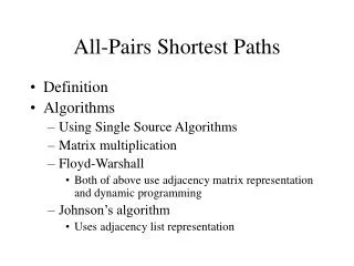
Dynamic programming algorithms for all-pairs shortest path and longest common subsequences • We will study a new technique—dynamic programming algorithms (typically for optimization problems) • Ideas: • Characterize the structure of an optimal solution • Recursively define the value of an optimal solution • Compute the value of an optimal solution in a bottom-up fashion (using matrix to compute) • Backtracking to construct an optimal solution from computed information.
Floyd-Warshall algorithm for shortest path: • Use a different dynamic-programming formulation to solve the all-pairs shortest-paths problem on a directed graph G=(V,E). • The resulting algorithm, known as the Floyd-Warshall algorithm, runs in O (V3) time. • negative-weight edges may be present, • but we shall assume that there are no negative-weight cycles.
The structure of a shortest path: • We use a different characterization of the structure of a shortest path than we used in the matrix-multiplication-based all-pairs algorithms. • The algorithm considers the “intermediate” vertices of a shortest path, where an intermediate vertex of a simple path p=<v1,v2,…,vl> is any vertex in p other than v1 or vl, that is, any vertex in the set {v2,v3,…,vl-1}
Continue: • Let the vertices of G be V={1,2,…,n}, and consider a subset {1,2,…,k} of vertices for some k. • For any pair of vertices i,j V, consider all paths from i to j whose intermediate vertices are all drawn from {1,2,…,k},and let p be a minimum-weight path from among them. • The Floyd-Warshall algorithm exploits a relationship between path p and shortest paths from i to j with all intermediate vertices in the set {1,2,…,k-1}.
Relationship: • The relationship depends on whether or not k is an intermediate vertex of path p. • If k is not an intermediate vertex of path p, then all intermediate vertices of path p are in the set {1,2,…,k-1}. Thus, a shortest path from vertex i to vertex j with all intermediate vertices in the set {1,2,…,k-1} is also a shortest path from i to j with all intermediate vertices in the set {1,2,…,k}. • If k is an intermediate vertex of path p,then we break p down into i k j as shown Figure 2.p1 is a shortest path from i to k with all intermediate vertices in the set {1,2,…,k-1}, so as p2.
All intermediate vertices in {1,2,…,k-1} p2 p1 k j i P:all intermediate vertices in {1,2,…,k} Figure 2. Path p is a shortest path from vertex i to vertex j,and k is the highest-numbered intermediate vertex of p. Path p1, the portion of path p from vertex i to vertex k,has all intermediate vertices in the set {1,2,…,k-1}.The same holds for path p2 from vertex k to vertex j.
A recursive solution to the all-pairs shortest paths problem: • Let dij(k) be the weight of a shortest path from vertex i to vertex j with all intermediate vertices in the set {1,2,…,k}. A recursive definition is given by • dij(k)= wij if k=0, • min(dij(k-1),dik(k-1)+dkj(k-1)) if k 1. • The matrix D(n)=(dij(n)) gives the final answer-dij(n)= for all i,j V-because all intermediate vertices are in the set {1,2,…,n}.
Computing the shortest-path weights bottom up: • FLOYD-WARSHALL(W) • n rows[W] • D(0) W • for k1 to n • dofor i 1 to n • do for j 1 to n • dij(k) min(dij(k-1),dik(k-1)+dkj(k-1)) • return D(n)
Example: • Figure 3 2 4 3 1 3 8 1 -5 -4 2 7 5 4 6
D(0)= (0)= (1)= D(1)=
D(2)= (2)= (3)= D(3)=
D(4)= (4)= (5)= D(5)=
Comparison of two strings • Longest common subsequence • Shortest common supersequence • Edit distance between two sequences
1. Longest common subsequence • Definition 1: Given a sequence X=x1x2...xm, another sequence Z=z1z2...zk is a subsequence of X if there exists a strictly increasing sequence i1i2...ik of indices of X such that for all j=1,2,...k, we have xij=zj. • Example 1: If X=abcdefg, Z=abdg is a subsequence of X. X=abcdefg,Z=ab d g
Definition 2: Given two sequences X and Y. A sequence Z is a common subsequence of X and Y if Z is a subsequence of both X and Y. • Example 2: X=abcdefg and Y=aaadgfd. Z=adf is a common subsequence of X and Y. X=abc defg Y=aaaadgfd Z=a d f
Definition 3: A longest common subsequence of X and Y is a common subsequence of X and Y with the longest length. (The length of a sequence is the number of letters in the seuqence.) • Longest common subsequence may not be unique.
Longest common subsequence problem • Input: Two sequences X=x1x2...xm, and Y=y1y2...yn. • Output: a longest common subsequence of X and Y. • A brute-force approach Suppose that mn. Try all subsequence of X (There are 2m subsequence of X), test if such a subsequence is also a subsequence of Y, and select the one with the longest length.
Charactering a longest common subsequence • Theorem (Optimal substructure of an LCS) • Let X=x1x2...xm, and Y=y1y2...yn be two sequences, and • Z=z1z2...zk be any LCS of X and Y. • 1. If xm=yn, then zk=xm=yn and Z[1..k-1] is an LCS of X[1..m-1] and Y[1..n-1]. • 2. If xmyn, then zkxm implies that Z is an LCS of X[1..m-1] and Y. • 2. If xmyn, then zkyn implies that Z is an LCS of X and Y[1..n-1].
The recursive equation • Let c[i,j] be the length of an LCS of X[1...i] and X[1...j]. • c[i,j] can be computed as follows: 0 if i=0 or j=0, c[i,j]= c[i-1,j-1]+1 if i,j>0 and xi=yj, max{c[i,j-1],c[i-1,j]} if i,j>0 and xiyj. Computing the length of an LCS • There are nm c[i,j]’s. So we can compute them in a specific order.
The algorithm to compute an LCS • 1. for i=1 to m do • 2. c[i,0]=0; • 3. for j=0 to n do • 4. c[0,j]=0; • 5. for i=1 to m do • 6. for j=1 to n do • 7. { • 8. if xi ==yj then • 9. c[i,j]=c[i-1,j-1]=1; • 10 b[i,j]=1; • 11. elseif c[i-1,j]>=c[i,j-1] then • 12. c[i,j]=c[i-1,j] • 13. b[i,j]=2; • 14. else c[i,j]=c[i,j-1] • 15. b[i,j]=3; • 14 }
Constructing an LCS (back-tracking) • We can find an LCS using b[i,j]’s. • We start with b[n,m] and track back to some cell b[0,i] or b[i,0]. • The algorithm to construct an LCS 1. i=m 2. j=n; 3. if i==0 or j==0 then exit; 4. if b[i,j]=1 then { i=i-1; j=j-1; print “xi”; } 5. if b[i,j]==2 i=i-1 6. if b[i,j]==3 j=j-1 7. Goto Step 3. • The time complexity: O(nm).
2. Shortest common supersequence • Definition: Let X and Y be two sequences. A sequence Z is a supersequence of X and Y if both X and Y are subsequence of Z. • Shortest common supersequence problem: Input: Two sequences X and Y. Output: a shortest common supersequence of X and Y.
Recursive Equation: • Let c[i,j] be the length of an LCS of X[1...i] and X[1...j]. • c[i,j] can be computed as follows: j if i=0 i if j=0, c[i,j]= c[i-1,j-1]+1 if i,j>0 and xi=yj, min{c[i,j-1]+1,c[i-1,j]+1} if i,j>0 and xiyj.
3. Edit distance between two sequences Three operations: • insertion: inserting an x into abc (between a and b), we get axbc. • deletion: deleting b from abc, we get ac. • replacement: Given a sequence abc, replacing a with x, we get xbc.
Definition: Suppose that we can use three edit operations (insertion, deletion, and replacement) to edit a sequence into another. The edit distance between two sequences is the minimum number of operations required to edit one sequence into another. • Note: each operation is counted as 1. Weighted edit distance: • There is a weight on each operation. • For example: s(a,b)=1, s(a, _)=1.5, s(b,a)=1, s(b,_)=1.5. • Where the weight comes from: • For DNA and protein sequences, it is from statistics.
Alignment of sequences -- an alternative • An alignment of two sequences is obtained by inserting spaces into or at either end of X and Ysuch that the two resulting sequences X’ and Y’ are of the same length. That is, every letter in X’ is opposite to a unique letter in Y’. • The alignment value is defined as • where X’[i] and Y’[i] denote the two letters in column i of the alignment and s(X’[i], Y’[i]) is the score (weight) of these opposing letters. • There are several popular socre schemes for DNA and protein sequences.
Facts: The edit distance between two sequences is the same as the alignment value of two sequences if we use the same score scheme. • Recursive equation: c[i,j]=min{ c[i-1, j-1]+s(X[i], Y[j]), c[i, j-1]+s(_,Y[j]), c[i-1, j)+s(X[i],_)}. • Time and space complexity Both are O(nm) or O(n2) if both sequences have equal length n. • Why? We have to compute c[i,j] (the cost) and b[i,j] (for back-tracking). Each will take O(n2).
Linear space algorithm • Hints: Computing c[i,j] needs linear space whereas back-tracking needs O(nm) time.
To compute c[i,j], we need c[i-1,j-1], c[i,j-1], & c[i-1,j]. • So, to get c[n,m], we only have to keep dark cells. • However, if we do not have all the b[i,j]’s, we can not get the alignment (nor the edit process, the subsequence, the supersequence).
Discussion: Each time we only keep a few b[i,j]’s and we can re-compute the b[i,j]’s again. In this way, we can get a linear space algorithm. However, the time complexity is increased to O(n3).
A Better Idea: find a cuting point. • For the problems of smaller size, we do the same thing until one of the segment contains 1 letter. • Key: each time, we fix the middle point (n/2) of X.
Example: X=abcdefgh and Y=aacdefhh. • Score scheme: match -- 0 and mismatch -- 1. The alignment abcdefgh abcd efgh aacdefhh aacd efhh /|\ cutting point (4,4).
Finding the cutting point: Let X=x1x2x3...xn and Y=y1y2y3...ym. Define XT=xnxn-1...x1 and YT=ymym-1 ...y1. Let c[i,j] be the cost of optimal alignment for X[1...i] and Y[1...j] and cc[k,l] be the cost of optimal alignment for XT[1...k] and YT[1...l]. for (i=1, i<=n i++) if( (c[[n/2], i]+cc[n-[n/2], m-i]) ==c[n,n]) point = i; We need to check two rows, c[[n/2],1], c[[n/2],2], ...c[[n/2],m] and cc[n-[n/2], 1], cc[n-[n/2],2], ... cc[n-[n/2],m]. O(m) space.
The algorithm 1. compute c[n,n], the [n/2]-th row and the ([n/2]+1)-th row of c. 2. find the cutting point ([n/2], i) as shown above. 3. if i-[n/2] == 1 then compute the alignment of X[1...[n/2]) and Y[1...i]. 4. if n-[n/2]+1 == 1 then compute the alignment of X[[n/2]+1...n] and Y[i+1...n]. 5. if i-[n/2] != 1 and n-[n/2]+1 !=1 then recursive on step 1-4 for the two pairs of sequences X[1...[n/2]) and Y[1...i], and X[[n/2]+1...n] and Y[i+1...n]; finally combine the two alignments for the two pairs of sequences.
Time complexity analysis: • The first round needs T’ time, where T’ is the time for the normal algorithm. (O(n2).) • 2nd round needs 1/2 T’. (0.5 n i +0.5 n (n-i)=0.5n2.) • 3rd round need 1/4 T’. • i-th round needs 1/2i-1 T’. • Total time T=(1/2+1/4+1/8+ ... )T’ =2T’ =O(n2).