Download
1 / 39
400 likes | 530 Views
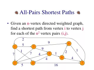
All-Pairs Shortest Paths. Find the distance between every pair of vertices in a weighted graph G. From A one may reach C faster by reaching by traveling from A to B and then from B to C. All-Pairs Shortest Paths. We can make n calls to Dijkstra’s algorithm O(n(n+m)log n) time.

E N D
All-Pairs Shortest Paths • Find the distance between every pair of vertices in a weighted graph G.
From A one may reach C faster by reaching by traveling from A to B and then from B to C. All-Pairs Shortest Paths • We can make n calls to Dijkstra’s algorithm • O(n(n+m)log n) time • Alternatively ... Use dynamic programming: The Floyd’s Algorithm • O(n3) time.
Floyd’s Shortest Path Algorithm • Idea #1: Number the vertices 1, 2, …, n. • Idea #2: Shortest path between vertex i and vertex j without passing through any other vertex is weight(edge(i,j)). • Let it be D0(i,j). • Idea #3: If Dk(i,j) is the shortest path between vertex i and vertex j using vertices numbered 1, 2, …, k, as intermediate vertices, then Dn(i,j) is the solution to the shortest path problem between vertex i and vertex j.
Uses only vertices numbered 1,…,k (compute weight of this edge) i j Uses only vertices numbered 1,…,k-1 Uses only vertices numbered 1,…,k-1 k Floyd’s Shortest Path Algorithm • Assume that we have Dk-1(i,j) for all i, and j. • We wish to compute Dk(i,j). • What are the possibilities? Choose between • a path through vertex k. • Path Length: Dk(i,j) = Dk-1(i,k) + Dk-1(k,j). • (2) Skip vertex k altogether. • Path Length: Dk(i,j) = Dk-1(i,j).
Floyd’s Shortest Path Algorithm Uses only vertices numbered 1,…,k (compute weight of this edge) i j Uses only vertices numbered 1,…,k-1 k Uses only vertices numbered 1,…,k-1
Floyd’s Shortest Path Algorithm Example: 8 D0 1 2 4 3 1 3 2 1 1 5 4 8
Floyd’s Shortest Path Algorithm Example: 8 D1 1 2 4 3 1 3 2 1 1 5 4 8
Floyd’s Shortest Path Algorithm Example: 8 D2 1 2 4 3 1 3 2 1 1 5 4 8
Floyd’s Shortest Path Algorithm Example: 8 D3 1 2 4 3 1 3 2 1 1 5 4 8
Floyd’s Shortest Path Algorithm Example: 8 D4 1 2 4 3 1 3 2 1 1 5 4 8
Floyd’s Shortest Path Algorithm Example: 8 D5 1 2 4 3 1 3 2 1 1 5 4 8
Floyd’s Shortest Path Algorithm AlgorithmAllPair(G) {assumes vertices 1,…,n} for allvertex pairs (i,j) ifi= j d0[i,i] 0 else if (i,j)is an edge in G d0[i,j] weight of edge (i,j) elsed0[i,j] + fork 1 to n do fori 1 to n do forj 1 to n do dk[i,j] min(dk-1[i,j], dk-1[i,k]+dk-1[k,j]) O(n+m) or O(n2) O(n3)
Floyd’s Shortest Path Algorithm Observation: dk [i,k] = dk-1[i,k] dk[k,j] = dk-1[k,j]
Floyd’s Shortest Path Algorithm AlgorithmAllPair(G) {assumes vertices 1,…,n} for allvertex pairs (i,j) ifi= j d[i,i] 0 else if (i,j)is an edge in G d[i,j] weight of edge (i,j) elsed[i,j] + fork 1 to n do fori 1 to n do forj 1 to n do d[i,j] min(d[i,j], d[i,k]+d[k,j])
Floyd’s Shortest Path Algorithm AlgorithmAllPair(G) {assumes vertices 1,…,n} for allvertex pairs (i,j) path[i,j] null ifi= j d[i,i] 0 else if (i,j)is an edge in G d[i,j] weight of edge (i,j) elsed[i,j] + fork 1 to n do fori 1 to n do forj 1 to n do if (d[i,k]+d[k,j] < d[i,j]) path[i,j] vertexk d[i,j] d[i,k]+d[k,j]
Floyd’s Shortest Path Algorithm • Can be applied to Directed Graphs • Can accept –ve edges as long as there are no –ve cycles.
Transitive Closure • Transitive Relation: A relation R on a set A is called transitive if and only if for any a, b, and c in A, whenever <a, b> R , and <b, c> R ,<a, c> R
D E B C A Transitive Closure D E • Given a graph G, the transitive closure of G is the G* such that • G* has the same vertices as G • if G has a path from u to v (u v), G* has a edge from u to v B G C A The transitive closure provides reachability information about a graph. G*
If there's a way to get from A to B and from B to C, then there's a way to get from A to C. Computing the Transitive Closure • We can perform BFS starting at each vertex • O(n(n+m)) Alternatively ... Use dynamic programming: Warshall’s Algorithm
Floyd-Warshall Transitive Closure • Idea #1: Number the vertices 1, 2, …, n. • Idea #2: Consider paths that use only vertices numbered 1, 2, …, k, as intermediate vertices: Uses only vertices numbered 1,…,k (add this edge if it’s not already in) i j Uses only vertices numbered 1,…,k-1 Uses only vertices numbered 1,…,k-1 k
Warshall’s Transitive Closure Example: A0 1 2 3 4
Warshall’s Transitive Closure Example: A1 1 2 3 4
Warshall’s Transitive Closure Example: A2 1 2 3 4
Warshall’s Transitive Closure Example: A3 1 2 3 4
Warshall’s Transitive Closure Example: A4 1 2 3 4
Warshall’s Algorithm AlgorithmFloydWarshall(G) Inputgraph G Outputtransitive closure G* of G i 1 for all v G.vertices() denote v as vi i i+1 G0G for k 1 to n do GkGk -1 for i 1 to n (i k)do for j 1 to n (j i, k)do if Gk -1.areAdjacent(vi, vk) Gk -1.areAdjacent(vk, vj) if Gk.areAdjacent(vi, vj) Gk.insertEdge(vi, vj , k) return Gn • Warshall’s algorithm numbers the vertices of G as v1 , …, vn and computes a series of graphs G0, …, Gn • G0=G • Gkhas a edge (vi, vj) if G has a path from vi to vjwith intermediate vertices in the set {v1 , …, vk} • We have that Gn = G* • In phase k, graph Gk is computed from Gk -1 • Running time: O(n3), assuming areAdjacent is O(1) (e.g., adjacency matrix)
Shortest Path Algorithm for DAGs • Use Dijkstra’s algorithm • Time: O((n+m) log n) • Use Topological sort based algorithm • Time: O(n+m).
Directed Graph With –ve weight $170 PVD -$100 ORD $28 SFO LGA -$100 -$200 $261 $68 $277 $511 HNL $210 $246 LAX $224 DFW MCO 0
Directed Graph With –ve weight $170 PVD 3 -$100 ORD 4 $28 SFO 8 LGA 2 -$100 -$200 $261 $68 $277 $511 HNL 7 $210 $246 LAX 6 $224 DFW 5 MCO 1 0
Directed Graph With –ve weight $170 PVD 3 -$100 ORD 4 $28 SFO 8 $224 LGA 2 -$100 -$200 $261 $68 $277 $511 HNL 7 $210 $210 $246 LAX 6 $224 DFW 5 MCO 1 $224 0
Directed Graph With –ve weight $170 PVD 3 -$100 ORD 4 $28 SFO 8 $261 LGA 2 -$100 -$200 $261 $68 $277 $511 HNL 7 $210 $210 $246 LAX 6 $224 DFW 5 MCO 1 $224 0
Directed Graph With –ve weight $170 PVD 3 -$100 ORD 4 $28 SFO 8 $238 LGA 2 -$100 -$200 $261 $68 $277 $511 HNL 7 $210 $210 $246 LAX 6 $224 DFW 5 MCO 1 $224 0
Directed Graph With –ve weight $170 PVD 3 -$100 ORD 4 $28 SFO 8 $238 $408 LGA 2 -$100 -$200 $261 $68 $277 $511 HNL 7 $210 $210 $246 LAX 6 $224 DFW 5 MCO 1 $224 0
Directed Graph With –ve weight $170 PVD 3 -$100 ORD 4 $28 SFO 8 $238 $408 LGA 2 -$100 $308 -$200 $261 $68 $277 $511 HNL 7 $210 $210 $246 LAX 6 $224 DFW 5 MCO 1 $208 $224 0
Directed Graph With –ve weight $170 PVD 3 -$100 ORD 4 $28 SFO 8 $238 $408 LGA 2 -$100 $308 -$200 $261 $68 $277 $511 HNL 7 $210 $210 $246 LAX 6 $224 DFW 5 MCO 1 $208 $224 0
Directed Graph With –ve weight $170 PVD 3 -$100 ORD 4 $28 SFO 8 $238 $408 LGA 2 -$100 $268 -$200 $261 $68 $277 $511 HNL 7 $210 $210 $246 LAX 6 $224 DFW 5 $719 MCO 1 $208 $224 0
Directed Graph With –ve weight $170 PVD 3 -$100 ORD 4 $28 SFO 8 $238 $408 LGA 2 -$100 $268 -$200 $261 $68 $277 $511 HNL 7 $210 $210 $246 LAX 6 $224 DFW 5 $719 MCO 1 $208 $224 0
Directed Graph With –ve weight $170 PVD 3 -$100 ORD 4 $28 SFO 8 $238 $408 LGA 2 -$100 $268 -$200 $261 $68 $277 $511 HNL 7 $210 $210 $246 LAX 6 $224 DFW 5 $719 MCO 1 $208 $224 0
DAG-based Algorithm AlgorithmDagDistances(G, s) for allv G.vertices() v.parent null ifv= s v.distance 0 else v.distance Perform a topological sort of the vertices foru 1 to n do{in topological order} for eache G.outEdges(u) w G.opposite(u,e) r getDistance(u) + weight(e) ifr< getDistance(w) w.distance r w.parent u • Works even with negative-weight edges • Uses topological order • Doesn’t use any fancy data structures • Is much faster than Dijkstra’s algorithm • Running time: O(n+m).