Download

1 / 32
320 likes | 613 Views
Shortest Path Algorithms. Andreas Klappenecker [based on slides by Prof. Welch]. s. t. Single Source Shortest Path Problem. Given: a directed or undirected graph G = (V,E), a source node s in V, and a weight function w: E -> R.

E N D
Shortest Path Algorithms Andreas Klappenecker [based on slides by Prof. Welch]
s t Single Source Shortest Path Problem • Given: a directed or undirected graph G = (V,E), a source node s in V, and a weight function w: E -> R. • Goal: For each vertex t in V, find a path from s to t in G with minimum weight Warning! Negative weight cycles are a problem: 4 5
Constant Weight Functions Suppose that the weights of all edges are the same. How can you solve the single-source shortest path problem? Breadth-first search can be used to solve the single-source shortest path problem. Indeed, the tree rooted at s in the BFS forest is the solution.
Priority Queues A min-priority queue is a data structure for maintaining a set S of elements, each with an associated value called key. This data structure supports the operations: • insert(S,x)which realizes S := S {x} • minimum(S) which returns the element with the smallest key. • extract-min(S) which removes and returns the element with the smallest key from S. • decrease-key(S,x,k) which decreases the value of x’s key to the lower value k, where k < key[x].
Simple Array Implementation Suppose that the elements are numbered from 1 to n, and that the keys are stored in an array key[1..n]. • insert and decrease-key take O(1) time. • extract-min takes O(n) time, as the whole array must be searched for the minimum.
Binary min-heap Implementation Suppose that we realize the priority queue of a set with n element with a binary min-heap. • extract-min takes O(log n) time. • decrease-key takes O(log n) time. • insert takes O(log n) time. Building the heap takes O(n) time.
Fibonacci-Heap Implementation Suppose that we realize the priority queue of a set with n elements with a Fibonacci heap. Then • extract-min takes O(log n) amortized time. • decrease-key takes O(1) amortized time. • insert takes O(1) time. [One can realize priority queues with worst case times as above]
Dijkstra's SSSP Algorithm • Assumes all edge weights are nonnegative • Similar to Prim's MST algorithm • Start with source node s and iteratively construct a tree rooted at s • Each node keeps track of tree node that provides cheapest path from s (not just cheapest path from any tree node) • At each iteration, include the node whose cheapest path from s is the overall cheapest
4 5 1 s 6 Prim's MST Prim's vs. Dijkstra's 4 5 1 s 6 Dijkstra's SSSP
Implementing Dijkstra's Alg. • How can each node u keep track of its best path from s? • Keep an estimate, d[u], of shortest path distance from s to u • Use d as a key in a priority queue • When u is added to the tree, check each of u's neighbors v to see if u provides v with a cheaper path from s: • compare d[v] to d[u] + w(u,v)
Dijkstra's Algorithm • input: G = (V,E,w) and source node s // initialization • d[s] := 0 • d[v] := infinity for all other nodes v • initialize priority queue Q to contain all nodes using d values as keys
Dijkstra's Algorithm • while Q is not empty do • u := extract-min(Q) • for each neighbor v of u do • if d[u] + w(u,v) < d[v] then // relax • d[v] := d[u] + w(u,v) • decrease-key(Q,v,d[v]) • parent(v) := u
Dijkstra's Algorithm Example iteration 2 a b 12 8 4 c 10 9 6 3 2 d e 4 a is source node
Correctness of Dijkstra's Alg. • Let Ti be the tree constructed after i-th iteration of the while loop: • The nodes in Ti are not in Q • The edges in Ti are indicated by parent variables • Show by induction on i that the path in Ti from s to u is a shortest path and has distance d[u], for all u in Ti. • Basis: i = 1. s is the only node in T1 and d[s] = 0.
Ti+1 Ti s x u Correctness of Dijkstra's Alg. • Induction: Assume Ti is a correct shortest path tree. We need to show that Ti+1 is a correct shortest path tree as well. • Let u be the node added in iteration i. • Let x = parent(u). Need to show path in Ti+1 from s to u is a shortest path, and has distance d[u]
P', another path from s to u a s x u b Correctness of Dijkstra's Alg P, path in Ti+1 from s to u Ti Ti+1 (a,b) is first edge in P' that leaves Ti
Correctness of Dijkstra's Alg Let P1 be part of P' before (a,b). Let P2 be part of P' after (a,b). w(P') = w(P1) + w(a,b) + w(P2) ≥ w(P1) + w(a,b) (nonneg wts) ≥ wt of path in Ti from s to a + w(a,b) (inductive hypothesis) ≥ w(s->x path in Ti) + w(x,u) (alg chose u in iteration i and d-values are accurate, by inductive hypothesis = w(P). So P is a shortest path, and d[u] is accurate after iteration i+1. Ti P Ti+1 s u x a b P'
Running Time of Dijstra's Alg. • initialization: insert each node once • O(V Tins) • O(V) iterations of while loop • one extract-min per iteration => O(V Tex) • for loop inside while loop has variable number of iterations… • For loop has O(E) iterations total • one decrease-key per iteration => O(E Tdec) • Total is O(V (Tins + Tex) + E Tdec)
Running Time using Binary Heaps and Fibonacci Heaps • O(V(Tins + Tex) + ETdec) • If priority queue is implemented with a binary heap, then • Tins = Tex = Tdec = O(log V) • total time is O(E log V) • There are fancier implementations of the priority queue, such as Fibonacci heap: • Tins = O(1), Tex = O(log V), Tdec = O(1) (amortized) • total time is O(V log V + E)
Using Simpler Heap Implementations • O(V(Tins + Tex) + ETdec) • If graph is dense, so that |E| = (V2), then it doesn't help to make Tins and Tex to be at most O(V). • Instead, focus on making Tdec be small, say constant. • Implement priority queue with an unsorted array: • Tins = O(1), Tex = O(V), Tdec = O(1) • total is O(V2)
What About Negative Edge Weights? • Dijkstra's SSSP algorithm requires all edge weights to be nonnegative. This is too restrictive, since it suffices to outlaw negative weight cycles. • Bellman-Ford SSSP algorithm can handle negative edge weights. [It even can detect negative weight cycles if they exist.]
Bellman-Ford: The Basic Idea • Consider each edge (u,v) and see if u offers v a cheaper path from s • compare d[v] to d[u] + w(u,v) • Repeat this process |V| - 1 times to ensure that accurate information propgates from s, no matter what order the edges are considered in
Bellman-Ford SSSP Algorithm • input: directed or undirected graph G = (V,E,w) //initialization • initialize d[v] to infinity and parent[v] to nil for all v in V other than the source • initialize d[s] to 0 and parent[s] to s // main body • for i := 1 to |V| - 1 do • for each (u,v) in E do // consider in arbitrary order • if d[u] + w(u,v) < d[v] then • d[v] := d[u] + w(u,v) • parent[v] := u
Bellman-Ford SSSP Algorithm // check for negative weight cycles • for each (u,v) in E do • if d[u] + w(u,v) < d[v] then • output "negative weight cycle exists"
Running Time of Bellman-Ford • O(V) iterations of outer for loop • O(E) iterations of inner for loop • O(VE) time total
Correctness of Bellman-Ford Assume no negative-weight cycles. Lemma: d[v] is never an underestimate of the actual shortest path distance from s to v. Lemma: If there is a shortest s-to-v path containing at most i edges, then after iteration i of the outer for loop, d[v] is at most the actual shortest path distance from s to v. Theorem: Bellman-Ford is correct. This follows from the two lemmas and the fact that every shortest path has at most |V| - 1 edges.
s c a b Bellman-Ford Example process edges in order (c,b) (a,b) (c,a) (s,a) (s,c) 3 2 —4 4 1 Exercise!
Correctness of Bellman-Ford • Suppose there is a negative weight cycle. • Then the distance will decrease even after iteration |V| - 1 • shortest path distance is negative infinity • This is what the last part of the code checks for.
The Boost Graph Library The BGL contains generic implementations of all the graph algorithms that we have discussed: • Breadth-First-Search • Depth-First-Search • Kruskal’s MST algorithm • Prim’s MST algorithm • Strongly Connected Components • Dijkstra’s SSSP algorithm • Bellman-Ford SSSP algorithm I recommend that you gain experience with this useful library. Recommended reading: The Boost Graph Library by J.G. Siek, L.-Q. Lee, and A. Lumsdaine, Addison-Wesley, 2002.