Download
1 / 28
290 likes | 378 Views
Extending GIS with Statistical Models to Predict Marine Species Distributions. Zach Hecht-Leavitt NY Department of State Division of Coastal Resources. Offshore Planning. NY. Long Island. NJ. Goals. Predict the abundance of selected groundfish species as a function of :

E N D
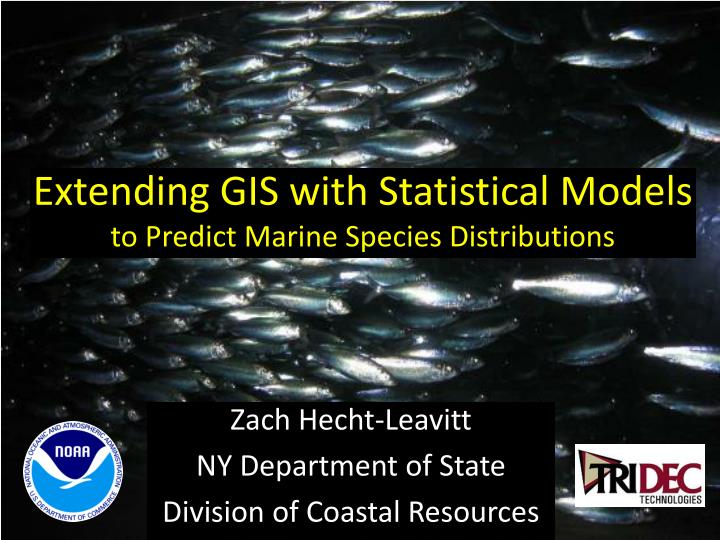
Extending GIS with Statistical Modelsto Predict Marine Species Distributions Zach Hecht-Leavitt NY Department of State Division of Coastal Resources
Offshore Planning NY Long Island NJ
Goals • Predict the abundance of selected groundfish species as a function of: • environmental/habitat variables • spatial autocorrelation • Assess error • Understand ecology
The Fish Data • NOAA Northeast Fisheries Science Center bottom trawl (catches groundfish) • Biannual 1975-2009 • Standardized gear, speed, and distance • Cleaned by Stone Environmental • Break down by season and life stage • 6 species selected NOAA NEFSC NOAA NEFSC
The Environmental Data • Depth • Distance from Shelf Edge • Bottom Grain Size • Slope • Sea Surface Temperature* • Chlorophyll* • Stratification* • Turbidity* • Zooplankton* • Provided by NOAA Biogeography Branch *Long-term, seasonal average
Data Exploration Adult Fluke Count • Approximate environmental relationships with lineartrend • Data is extremelyskewed (lots of zeroes) • Go with Zero-Inflated Generalized Linear Models (GLMs)
Workflow • “Loose” coupling • With 10.x can “hard” couple via Geospatial Modeling Environment (GME) Y=B1X1+B2X2… .CSV zeroinfl(), AchimZeileis
Workflow = + B2 * B1* B3 * +
The Residual -3 +5 -9 -1 +2 +3 +4 +1 -4 +2
Modeling Steps = + Predictors (GLM) + Residual (kriging) = Mean Expectation + Error (unexplained variation)
Error Assessment -4 +2 -1 -3 +2 +3
Error Assessment • 50/50 cross-validation • Smooth error with moving window • Final maps based on full dataset • Conservative error estimates
Final product (fluke example) M L L H L
Goals • Predict the abundance of selected groundfish as a function of: • environmental/habitat variables • spatial autocorrelation • Assess error • Understand ecology
Another Approach to Dealing with Zeroes
Another Approach • Rather than a one-size-fits all model… • … model presence/absence and abundance with two separate stages • May better reflect ecological reality • More conservative approach
Goals • Predict the abundance of selected cetaceans as a function of: • spatial autocorrelation • Assess error
The Marine Mammal Data • North Atlantic Right Whale Consortium Database • Aerial and shipboard surveys, 1978 - 2009 • Cleaned by New England Aquarium • SPUE • 4 species/groups selected • No predictors this time! NOAA SWFSC NOAA SWFSC
Stage I – Presence/Absence 1 1 4 1 1 5 1 2 1 0 0 0 1 1 1 1 1 1 3 4 1 1 4 1 2 0 0 0 3 1 0 0 0 0 0 0 0 4 2 0 0 0 0 1 1 0 0 0
Stage I – Presence/Absence 1 1 1 0 1 1 1 0 0 0 ROC Curve Epi package, Carstensen et. al.
Goals • Predict the abundance of selected cetaceans as a function of: • spatial autocorrelation • Assess error
Further reading • Hengl, T., G.B.M. Heuvelink and D.G. Rossiter. 2007. About regression-kriging: From equations to case studies. Computers and Geosciences 33:1301-1315. • Wenger, S. J. and M. C. Freeman. 2008. Estimating Species Occurrence, Abundance, And Detection Probability Using Zero-Inflated Distributions. Ecology 89:2953-2959 • Monestiez, P., L. Dubroca, E. Bonnin, J.-P. Durbec, C. Guinet. 2006. Geostatistical modeling of spatial distribution of Balaenopteraphysalus in the Northwestern Mediterranean Sea from sparse count data and heterogeneous observation efforts. Ecological Modeling, 193: 615-628. • Menza, C., B.P. Kinlan, D.S. Dorfman, M. Poti and C. Caldow (eds.). 2012. A Biogeographic Assessment of Seabirds, Deep Sea Corals and Ocean Habitats of the New York Bight: Science to Support Offshore Spatial Planning. NOAA Technical Memorandum NOS NCCOS 141. Silver Spring, MD. 224 pp.
Thank you! Zach.Hecht-Leavitt@dos.ny.gov / zhechtle@gmail.com