Download
1 / 42
420 likes | 576 Views
Algorithmentheorie 02 - Polynomprodukt und Fast Fourier Transformation. Prof. Dr. S. Albers Prof. Dr. Th. Ottmann. 1. Polynome. Reelles Polynom p in einer Variablen x p(x) = a n x n + ... +a 1 x 1 + a 0 a 0 ,..., a n R , a n 0: Koeffizienten von p

E N D
Algorithmentheorie02 - Polynomprodukt und Fast Fourier Transformation Prof. Dr. S. Albers Prof. Dr. Th. Ottmann WS 03/04
1. Polynome Reelles Polynompin einer Variablenx p(x) = anxn + ... +a1x1 + a0 a0 ,...,an R, an 0: Koeffizienten von p Grad von p: höchste Potenz in p(= n) Beispiel: p(x) = 3x3 – 15x2 + 18x Menge aller reellen Polynome: R[x] WS 03/04
2. Operationen auf Polynomen 1. Addition WS 03/04
Operationen auf Polynomen 2. Produkt c i: Welche Monomprodukte haben Grad i? Polynomring R[x] WS 03/04
Operationen auf Polynomen 3. Auswerten an der Stelle x0: Horner-Schema Zeit: O(n) WS 03/04
3. Repräsentation eines Polynoms p(x)Î R[x] Möglichkeit zur Repräsentation von p(x): 1. Koeffizientendarstellung Beispiel: WS 03/04
Repräsentation eines Polynoms 2. Nullstellenprodukt p(x)Î R[x] Beispiel: WS 03/04
Repräsentation eines Polynoms 3.Punkt/Wertdarstellung Interpolationslemma Jedes Polynom p(x) aus R[x] vom Grad n ist eindeutig bestimmt durch n+1 Paare (xi, p(xi)), mit i = 0,...,n und xi xj für i j Beispiel: Das Polynom wird durch die Paare (0,0), (1,6), (2,0), (3,0) eindeutig festgelegt. WS 03/04
Operationen auf Polynomen p, qÎ R[x], Grad(p) = Grad(q) = n • Koeffizientendarstellung Addition: O(n) Produkt: O(n2) Auswertung an der Stelle x0: O(n) • Punkt/Wertdarstellung WS 03/04
Operationen auf Polynomen Addition: Zeit: O(n) Produkt: (Voraussetzung: n Grad(pq)) Zeit: O(n) Auswerten an der Stelle x´: ?? Umwandeln in Koeffizientendarstellung (Interpolation) WS 03/04
Polynomprodukt Berechnung des Produkts zweier Polynome p, q vom Grade < n p,q Grad n-1, n Koeffizienten Auswertung: 2nPunkt/Wertpaare und Punktweise Multiplikation 2nPunkt/Wertpaare Interpolation pqGrad 2n-2, 2n-1 Koeffizienten WS 03/04
Ansatz für Divide and Conquer Idee:(n sei gerade) WS 03/04
Repräsentation von p(x) Annahme: Grad(p) <n 3a. Werte an den n Potenzen der n-ten komplexen Haupteinheitswurzel Potenz von n (Einheitswurzeln): 1 = WS 03/04
Diskrete Fourier Transformation Werte von p für die n Potenzen von n legen p eindeutig fest, falls Grad(p)<n. Diskrete Fourier Transformation (DFT) Beispiel:n=4 WS 03/04
Auswertung an den Einheitswurzeln WS 03/04
Auswertung an den Einheitswurzeln WS 03/04
Polynomprodukt Berechnung des Produkts zweier Polynome p, q vom Grade < n p,q Grad n-1, n Koeffizienten Auswertung: 2nPunkt/Wertpaare und Punktweise Multiplikation 2nPunkt/Wertpaare Interpolation pqGrad 2n-2, 2n-1 Koeffizienten WS 03/04
4. Eigenschaften der Einheitswurzel bilden eine multiplikative Gruppe Kürzungslemma Für alle n > 0, 0 kn, und d > 0 gilt: Beweis: Folge: WS 03/04
Eigenschaften der Einheitswurzel Halbierungslemma Die Menge der Quadrate der 2n komplexen 2n-ten Einheitswurzeln ist gleich der Menge der n komplexen n-ten Einheitswurzeln Beweis: WS 03/04
Eigenschaften der Einheitswurzel Summationslemma Für alle n > 0, j 0 mit Beweis: WS 03/04
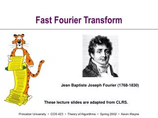
5. Diskrete Fourier Transformation Fast Fourier Transformation: Berechnung vonDFTn(p) mittels eines Divide-and-Conquer Ansatzes WS 03/04
Diskrete Fourier Transformation Idee:(n sei gerade) WS 03/04
Diskrete Fourier Transformation Auswertung für k = 0, ... , n – 1 WS 03/04
Beispiel: Diskrete Fourier Transformation WS 03/04
Berechnung von DFTn Einfachster Fall:n = 1 (Grad(p) = n –1 = 0) DFT1(p) = a0 Sonst : Divide: Teile p in p0und p1auf Conquer: Berechne DFTn/2(p0) und DFTn/2(p1) rekursiv Merge: Berechne für k = 0, ... , n –1: DFTn(p)k = WS 03/04
Eine kleine Verbesserung Also falls k < n/2: WS 03/04
Eine kleine Verbesserung Beispiel: WS 03/04
6. Fast Fourier Transformation AlgorithmusFFT Input: Ein Array a mit den n Koeffizienten eines Polynoms p und n = 2k Output:DFTn(p) 1. ifn = 1then /* p ist konstant */ 2.return a 3. d[0] = FFT([a0, a2, ... , an-2], n/2) 4. d[1] = FFT([a1, a3, ... , an-1], n/2) 5. n = e2i/n 6. = 1 • for k = 0to n/2 – 1do /* = nk*/ 11. returnd WS 03/04
FFT : Beispiel a = [0, 18,-15, 3 ] a[0] = [0, -15]a[1] = [18, 3] FFT([0, -15], 2) = (FFT([0],1) + FFT([-15],1), FFT([0],1) - FFT([-15],1)) = (-15,15) FFT([18, 3],2) = (FFT([18],1) + FFT([3],1), FFT([18],1) - FFT([3],1)) = (21,15) k = 0 ; = 1 d0 = -15 + 1 * 21 = 6d2 = -15 – 1* 21 = -36 k = 1 ; = i d1 = 15 + i*15 d3= 15 – i*15 FFT(a, 4) = (6, 15+15i,-36,15 –5i) WS 03/04
7. Analyse T(n) = Zeit um ein Polynom vom Grad < n an den Stellen auszuwerten. T(1) = O(1) T(n) = 2 T(n/2) + O(n) = O(n log n) WS 03/04
Polynomprodukt Berechnung des Produkts zweier Polynome p, q vom Grade < n p,q Grad n-1, n Koeffizienten Auswertung durch FFT: 2nPunkt/Wertpaare und Punktweise Multiplikation 2nPunkt/Wertpaare Interpolation pqGrad 2n-2, 2n-1 Koeffizienten WS 03/04
Interpolation Umrechnung der Punkt/Wert-Darstellung in die Koeffizientendarstellung Gegeben: (x0, y0),..., (xn-1, yn-1) mit xi xj, für alle i j Gesucht: Polynom p mit Koeffizienten a0,..., an-1, so dass WS 03/04
Interpolation Matrixschreibweise WS 03/04
Interpolation Spezialfall (hier) : Definition: WS 03/04
Interpolation Satz Für alle 0 i, j n – 1 gilt: Beweis zu zeigen: WS 03/04
Interpolation WS 03/04
Interpolation Fall 1:i = j Fall 2:i j, WS 03/04
Interpolation Summationslemma WS 03/04
Interpolation WS 03/04
Interpolation WS 03/04
Interpolation und DFT denn WS 03/04
Polynomprodukt durch FFT Berechnung des Produkts zweier Polynome p, q vom Grade < n p,q Grad n-1, n Koeffizienten Auswertung durch FFT: 2nPunkt/Wertpaare und Punktweise Multiplikation 2nPunkt/Wertpaare Interpolation durch FFT pqGrad 2n-2, 2n-1 Koeffizienten WS 03/04