Download
1 / 18
220 likes | 658 Views
Fast Fourier Transform. Irina Bobkova. Overview. I. Polynomials II. The DFT and FFT III. Efficient implementations IV. Some problems. Representation of polynomials. A polynomial in the variable x over an algebraic field F is representation of a function A(x) as a formal sum

E N D
Fast Fourier Transform Irina Bobkova
Overview I. Polynomials II. The DFT and FFT III. Efficient implementations IV. Some problems
Representation of polynomials • A polynomial in the variable x over an algebraic field F is representation of a function A(x) as a formal sum • Coefficient representation • Point-value representation
Interpolation-the inverse of evaluation –determining the coefficient form from a point-value representation Lagrange’s formula The coefficients can be computed in time Exercise. Prove it. Thus, n-point evaluation and interpolation are well-defined inverse operations between two representations. The algorithms described above for these problems take time . Interpolation
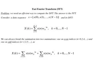
Fast multiplication Ordinary multiplication Time Θ(n²) Question.Can we use the linear-time multiplication method for polynomials in point-value form to expedite polynomial multiplication in coefficient form? Answer.Yes, but we are to be able to convert quickly from one form to another. Evaluation Time Θ(nlg n) Interpolation Time Θ(nlg n) Pointwise multiplication Time Θ(n)
Complex roots of unity There are exactly n complex roots of unity.They form a cyclic multiplication group: The value is called the primitive root of unity; all of the other complex roots are powers of it.
Discrete Fourier Transform Let F(x) be the polynomial with degree-bound n, which is a power of 2. is a primitive n-th root of unity. Let .Then The vector is called the Discrete Fourier Transform of vector a. The matrix is denoted by .
How to find Fn-1? Proposition. Let be a primitive l-th root of unity over a field L.Then Proof. The l =1 case is immediate since =1. Since is a primitive l-th root, each k ,k0 is a distinct l-th root of unity. Comparing the coefficients of Zl-1 on the left and right hand sides of this equation proves the proposition.
Inverse matrix to Fn Proposition. Let ω be an n-th root of unity.Then, Proof. The i=j case is obvious.If ij then will be a primitive root of unity of order l, where l|n.Applying the previous proposition completes the proof. So,
Fast Fourier Transform • So, the problem of evaluating A(x) reduces to: • Evaluating the degree-bound n/2 polynomials • 2. Combining the results
Time of the Recursive-FFT To determine the running time of procedure Recursive-FFT, we note, that exclusive of the recursive calls, each invocation takes time Θ(n), where n is the length of the input vector.The recurrence for the running time is therefore T(n) = 2T(n/2) + Θ(n) = Θ(n log n)
More effective implementations The for loop involves computing the value twice.We can change the loop(the butterfly operation): .
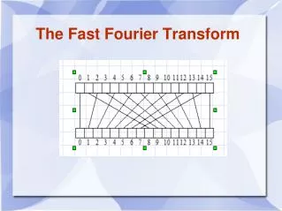
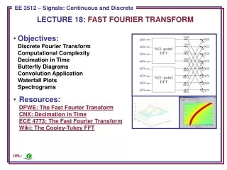
Iterative FFT 1) We take the elements in pairs, compute the DFT of each pair, using one butterfly operation, and replace the pair with its DFT 2) We take these n/2 DFT’s in pairs and compute the DFT of the four vector elements . . We take 2 (n/2)-element DFT’s and combine them using n/2 butterfly operations into the final n-element DFT
Iterative-FFT.Code. 0,4,2,6,1,5,3,7000,100,010,110,001,101,011,111000,001,010,011,100,101,110,111 BIT-REVERSE-COPY(a,A) nlength [a] for k0 to n-1 do A[rev(k)]ak ITERATIVE-FFT BIT-REVERSE-COPY(a,A) nlength [a] for s1 to log n do m2s m e2i/m for j0 to n-1 by m1 for j0 to m/2-1 do for kj to n-1 by m do t A[k+m/2] uA[k] A[k]u+t A[k+m/2]u-t m return A
A parallel FFT circuit a0 y0 a1 y1 a2 y2 a3 y3 a4 y4 a5 y5 a6 y6 a7 y7
Problem: evaluating all derivatives of a polynomial at a point Given coefficients b0,b1,…,bn-1 such that Show how to compute A(t) (x0), for t=0,1,2,…,n-1, in O(n) time. Explain how to find b0,b1,…,bn-1 in O(n lg n) time, given A( ) for k=0,1,2,…,n-1.
Problem: Toeplitz matrices A Toeplitz matrix is an n × n matrix , such that for i=2,3,…,n and j=2,3,…,n. Is the sum of two Toeplitz matrices necessarily Toeplitz? What about the product? Describe how to represent a Toeplitz matrix so that two n × n Toeplitz matrices can be added in O(n) time. Give an O(n lg n)-time algorithm for multiplying an n × n Toeplitz matrix by a vector of length n. Use your representation from part (b). Give an efficient algorithm for multiplying two n × n Toeplitz matrices. Analyze its running time.